Unsupervised Learning
Unsupervised learning algorithms identify patterns and relationships in data without predefined labels or outcomes. This section explores three key unsupervised techniques applied to the audio dataset: Principal Component Analysis (PCA) for dimensionality reduction, Clustering for grouping similar sounds, and Association Rule Mining (ARM) for discovering relationships between audio features.
Principal Component Analysis (PCA)
Principal Component Analysis (PCA) is a dimensionality reduction technique that transforms a dataset with potentially correlated variables into a set of linearly uncorrelated variables called principal components. These components are ordered by the amount of variance they explain in the original data, with the first component capturing the most variance. PCA helps us overcome the "curse of dimensionality," allowing for more efficient data visualization, pattern recognition, and computational processing while preserving the essential information in the data. The technique works by identifying the directions (principal components) where the data varies the most, projecting the data onto these new axes.
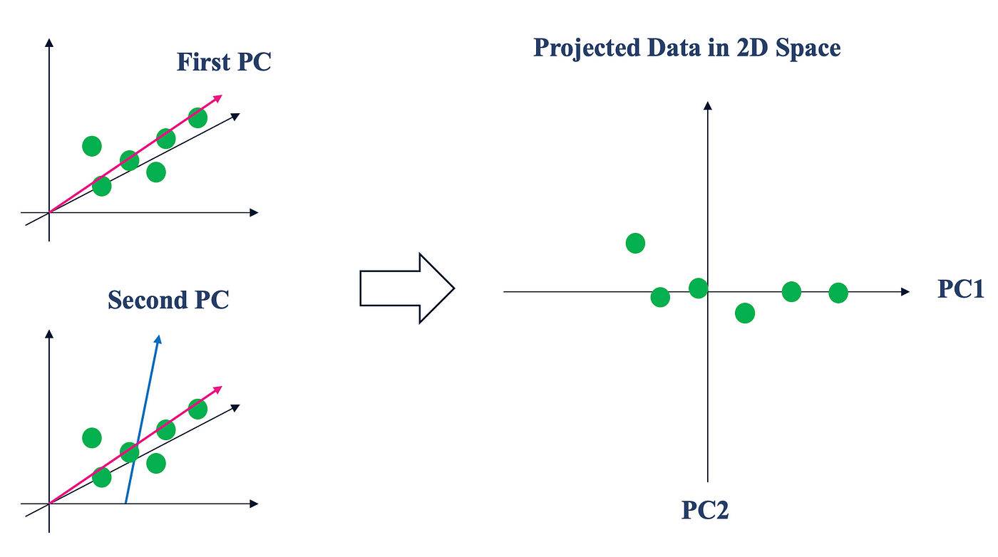
This diagram illustrates how PCA transforms high-dimensional data by projecting it onto new axes (principal components) that maximize variance. The first principal component (PC1) captures the direction of maximum variance, while subsequent components (PC2, PC3, etc.) capture remaining variance in orthogonal directions.
Understanding variance is key to PCA. In statistical terms, variance measures how spread out data points are from their mean. PCA finds the directions where the data varies the most, which typically contain the most important information. The first principal component points in the direction of maximum variance, essentially capturing the strongest pattern in the data. Each subsequent component is orthogonal (perpendicular) to the previous ones and captures the maximum remaining variance.
When we reduce dimensions using PCA, we can quantify how much information we retain through the "explained variance ratio" of each component. This tells us what percentage of the original data's variance is preserved by each principal component. Typically, we might keep enough components to retain 80-95% of the total variance, striking a balance between dimensionality reduction and information preservation.
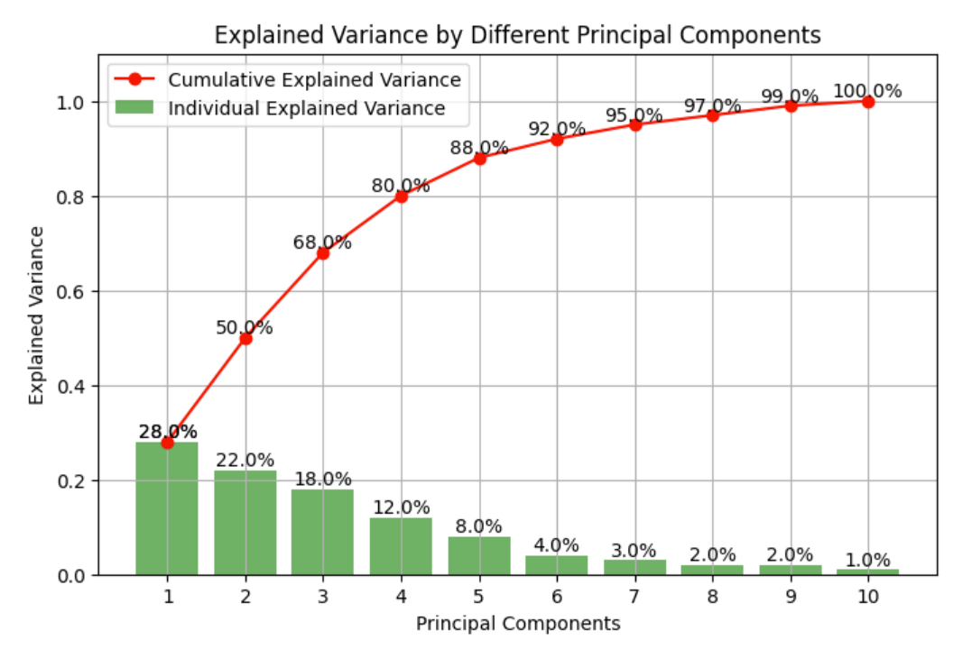
This chart shows a typical "explained variance ratio" plot for PCA. The bars represent how much variance each principal component explains, while the line shows the cumulative variance explained. This visualization helps in deciding how many components to retain for analysis.
PCA helped transform the numerous sound features into a smaller set of principal components that captured the essential patterns in the data. This revealed which combinations of sound characteristics were most important for distinguishing between different audio categories, eliminated redundant information, and made visualization and classification more effective.
Performing PCA on the Dataset
The original dataset contains 43 acoustic features extracted from approximately 15,000 audio samples across 20 sound categories. Each feature represents a different aspect of the audio signal, such as spectral characteristics, temporal patterns, and frequency content.
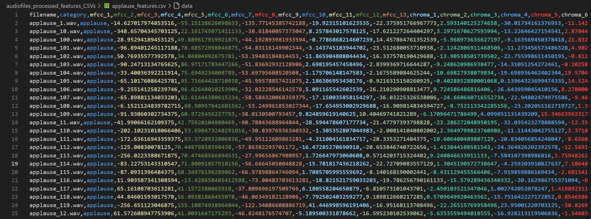
A preview of the original dataset showing the 43 acoustic features and category labels. Each row represents an audio sample, and each column represents a different acoustic feature. The second column as seen contains the sound category labels.
Before applying PCA, we needed to prepare the data by removing non-numeric features (category and filepath) and standardizing the remaining features. Standardization is crucial for PCA as it ensures that features with larger scales don't dominate the variance calculation. We used scikit-learn's StandardScaler to transform each feature to have zero mean and unit variance.
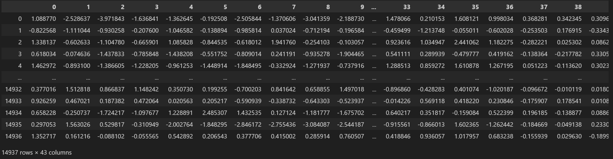
The processed dataset after removing categorical features and applying standardization. All features now have similar scales, allowing PCA to identify variance patterns based on actual data distribution rather than arbitrary feature scales.
After preparing the data, PCA was applied to reduce the 43-dimensional feature space to lower dimensions for visualization and further analysis. The full PCA transformed dataset is shown below.
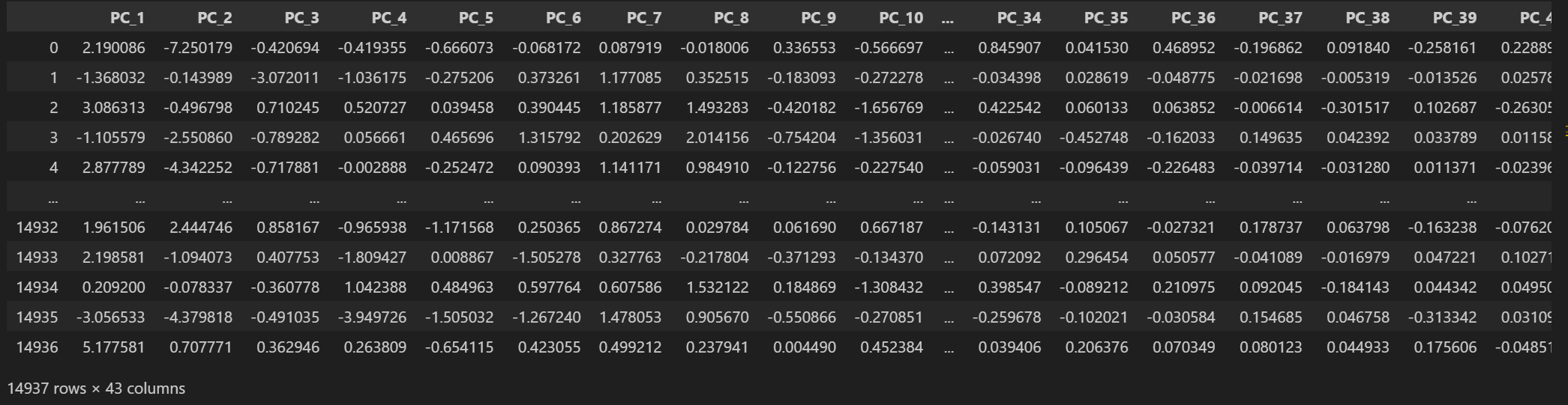
The 43 featured dataset is converted into 43 Principal components, with each successive component capturing less variance than the previous one.
The focus was on creating 2D and 3D representations that capture the most significant variance in the data while making it possible to visualize relationships between audio samples.
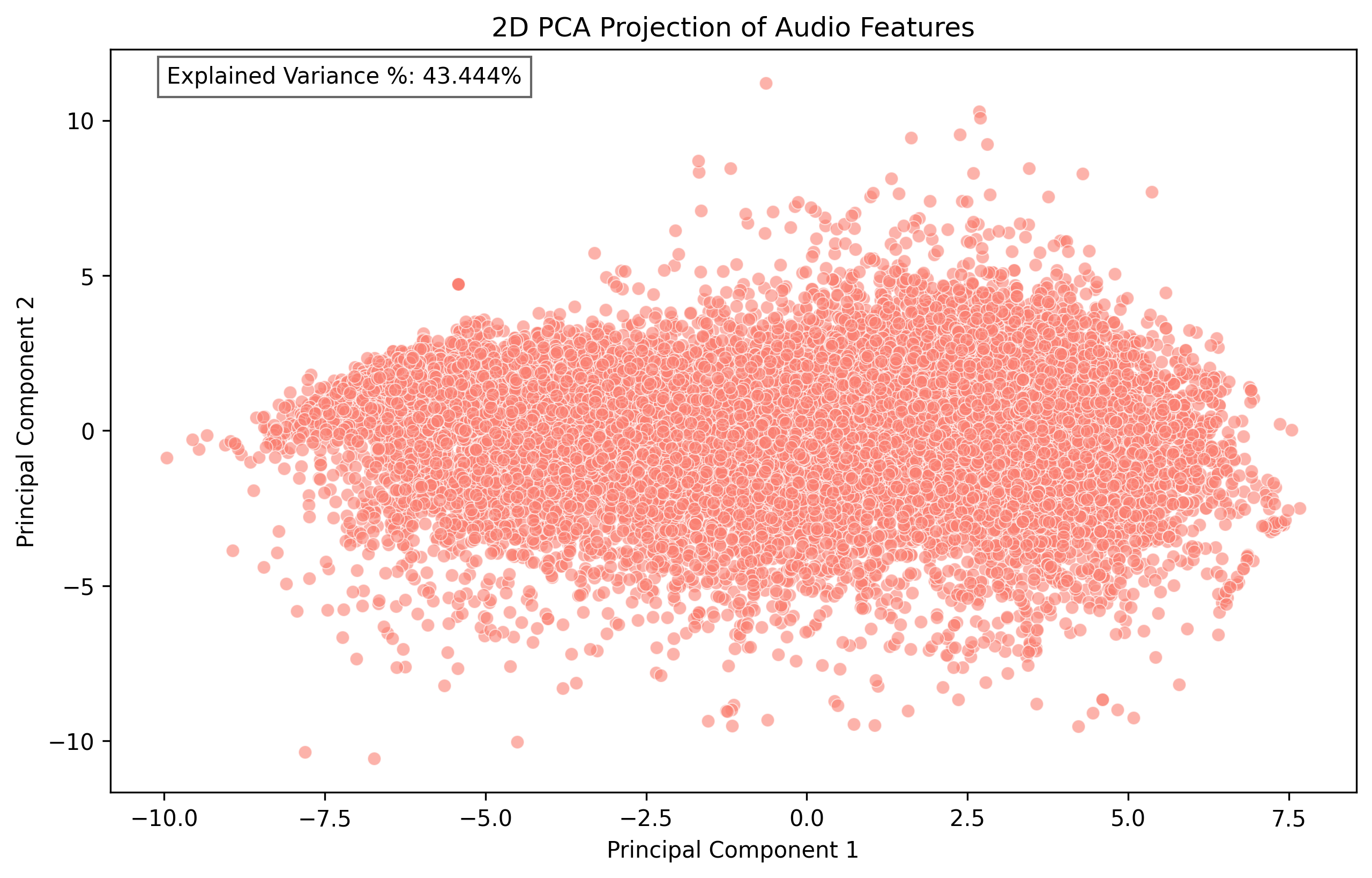
The 2D PCA visualization projects the audio samples onto the first two principal components, which together explain approximately 43% of the total variance.
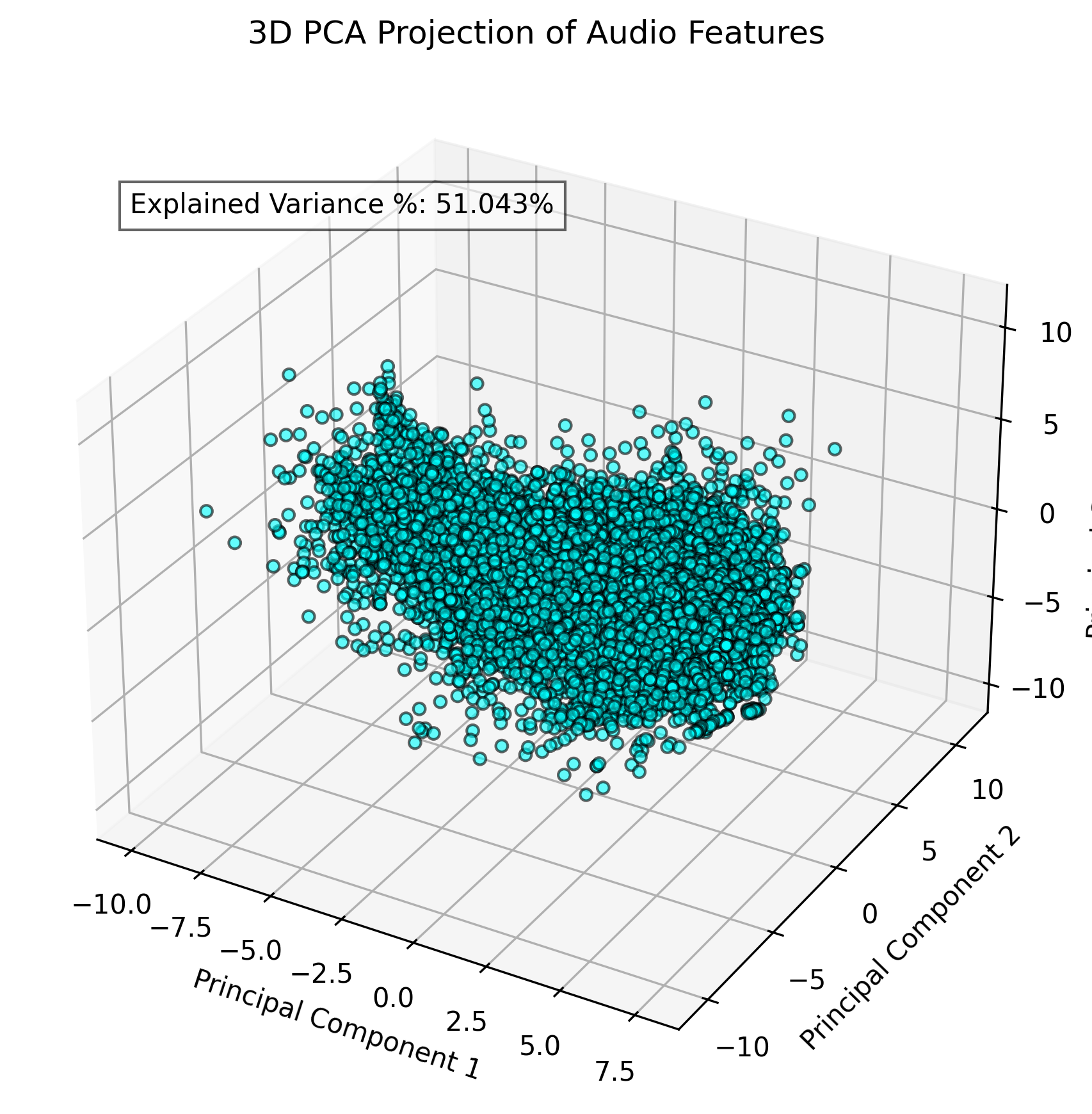
The 3D PCA visualization incorporates the third principal component, increasing the explained variance to approximately 51%.
Due to the high volume of data points, the standard PCA plots suffer from excessive clustering, obscuring the distinct patterns of individual categories. To address this limitation, we've implemented a customizable 3D PCA visualization tool that allows users to select specific categories of interest and control the sampling density, enabling clearer identification of categorical patterns and relationships within the feature space.
Custom PCA Visualization by Categories
Select one or more categories and specify the number of samples per category to generate a custom PCA visualization. This will help you compare how different sound categories are distributed in the PCA feature space.
Select Categories:
Samples per Category:
This custom PCA visualization displays the selected sound categories projected onto the principal components. Each color represents a different category, allowing for visual comparison of how different sounds cluster in the PCA space. The 2D view shows the first two principal components, while the 3D view adds the third component for additional dimensionality.
No categories selected yet. Select categories and generate the visualization to see the results.
Determining the Optimal Number of Components
To determine how many principal components should be retained for analysis, the explained variance ratio for each component was examined. This metric shows how much of the original data's variance is captured by each principal component.
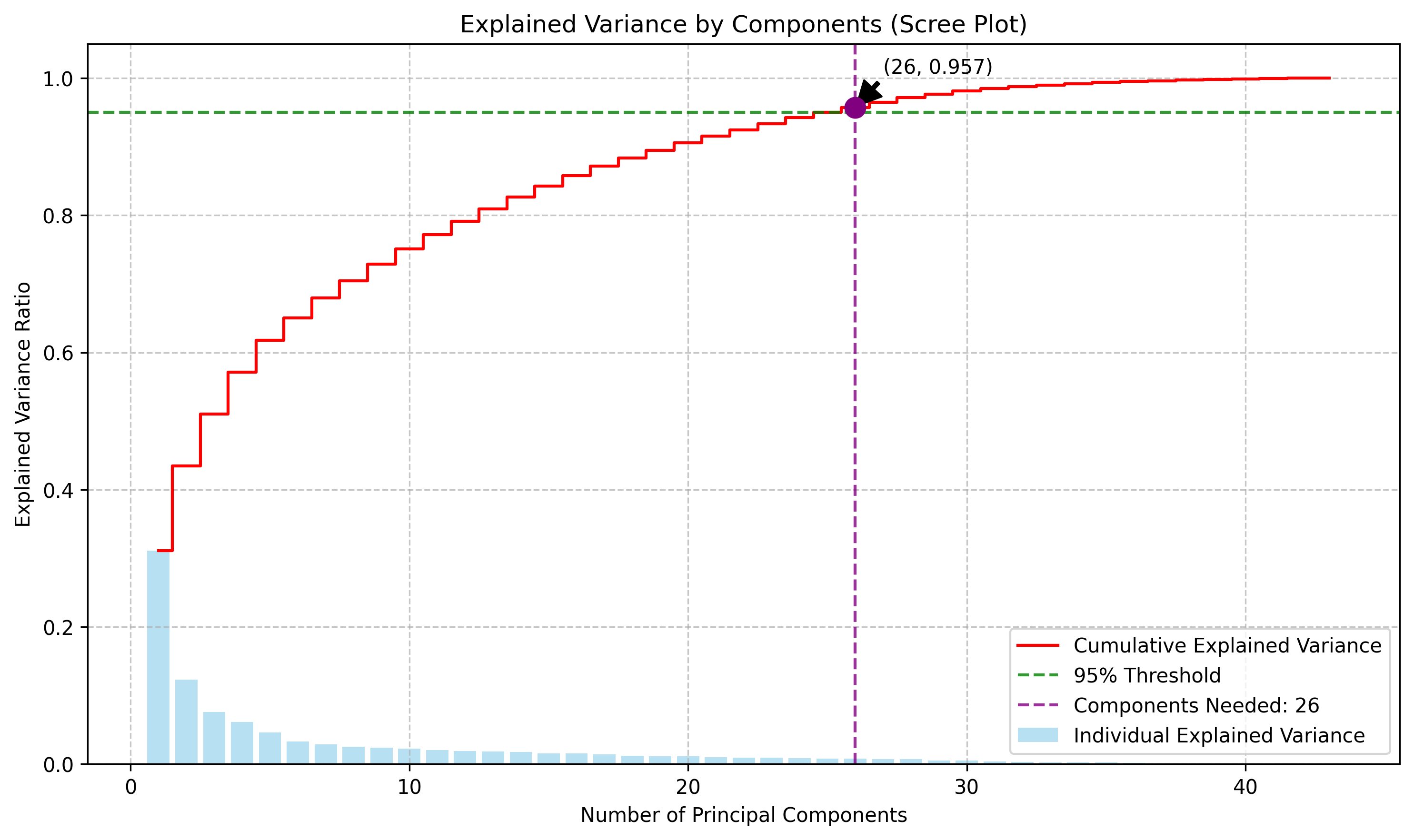
The cumulative explained variance plot shows that 26 principal components are needed to capture 95% of the total variance in the dataset. This represents a significant dimensionality reduction from the original 43 features while retaining most of the information, demonstrating PCA's effectiveness for the audio dataset.
Top Principal Components Analysis
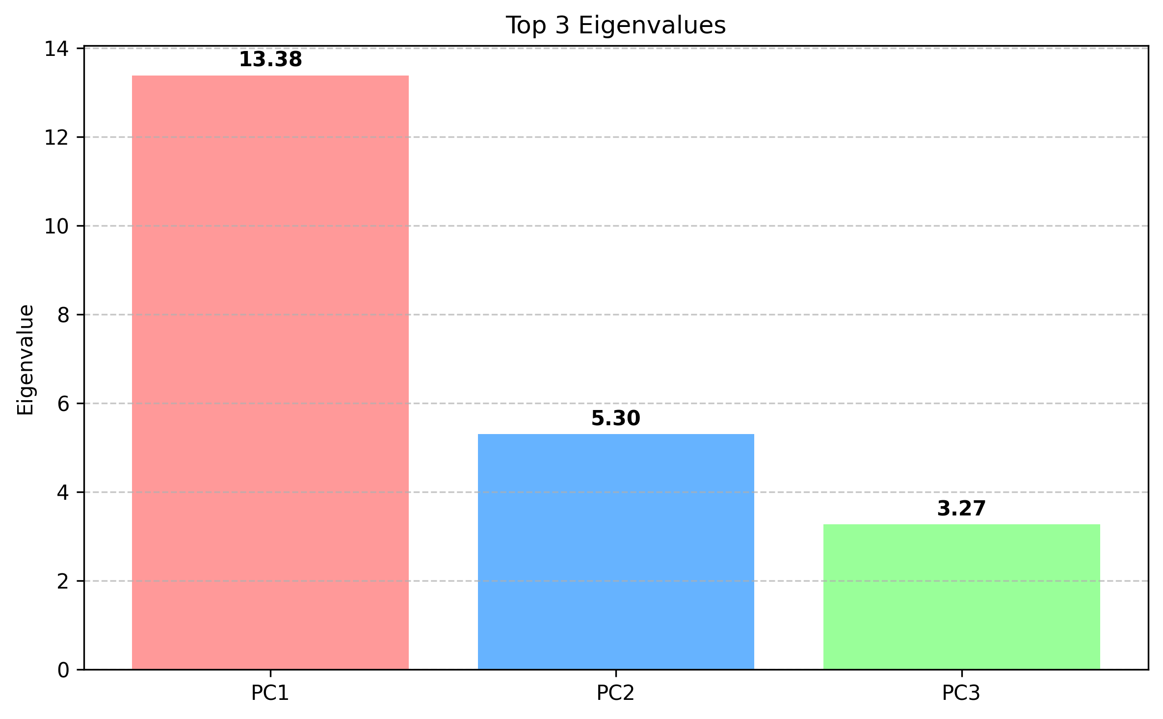
By examining the eigenvalues and eigenvectors of the top principal components, it becomes possible to understand which original features contribute most to the variance in the data. The top 3 eigenvalues are examined first.
We can now look at the contributions of the original features to the Principal Components.
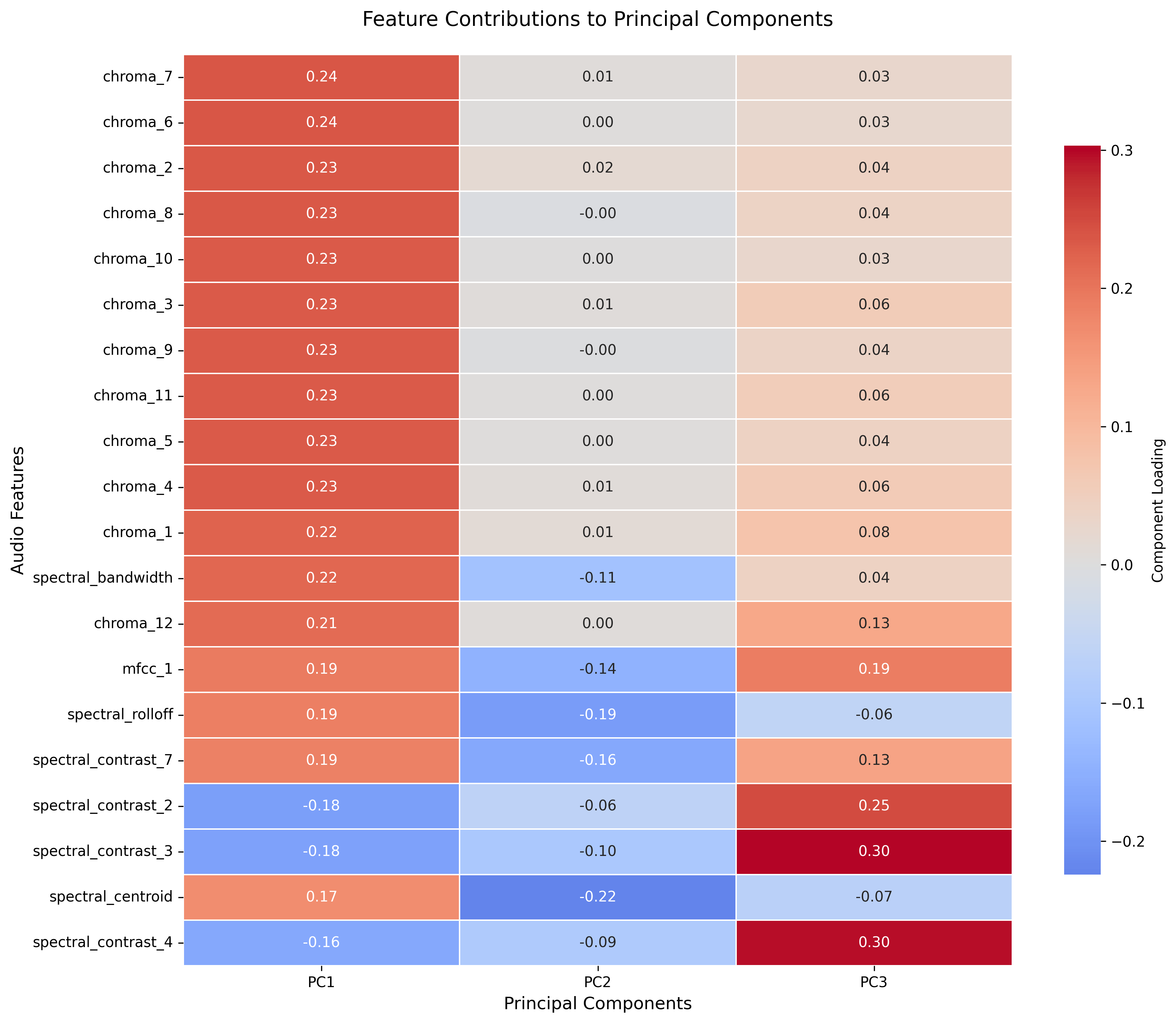
This visualization shows the top 15 contributing original feature to the three principal components. The first principal component is heavily influenced by chroma features, indicating that tonal information is crucial for distinguishing between sound categories. The second component is dominated by spectral features, while the third also shows significant contributions from spectral characteristics, suggesting the importance of these spectral properties for certain sound categories.
Conclusion
PCA has proven to be an invaluable tool for audio data analysis, allowing the reduction of the 43-dimensional feature space to a more manageable representation while preserving essential patterns. The 2D and 3D visualizations reveal natural groupings among sound categories that align with intuitive understanding of acoustic similarities. For instance, musical instruments cluster together, as do mechanical sounds and animal vocalizations. Moreover, PCA has prepared the data for more efficient clustering analysis by eliminating redundant information and noise. By focusing on the 26 principal components that capture 95% of the variance, the analysis can proceed with more computationally efficient and interpretable techniques while still retaining the most meaningful aspects of the sound features. For the sake of simplicity and visual clarity in the following sections, only 3 principal components are considered. The full script to perform PCA and its corresponding visualizations can be found here.
Clustering
Clustering is an unsupervised learning technique that groups similar data points together based on their inherent patterns and relationships, without predefined labels. The goal is to organize data into clusters where items within a cluster are more similar to each other than to those in other clusters. This similarity is typically measured using distance metrics such as Euclidean distance, Manhattan distance, or cosine similarity, which quantify how "close" data points are in the feature space.
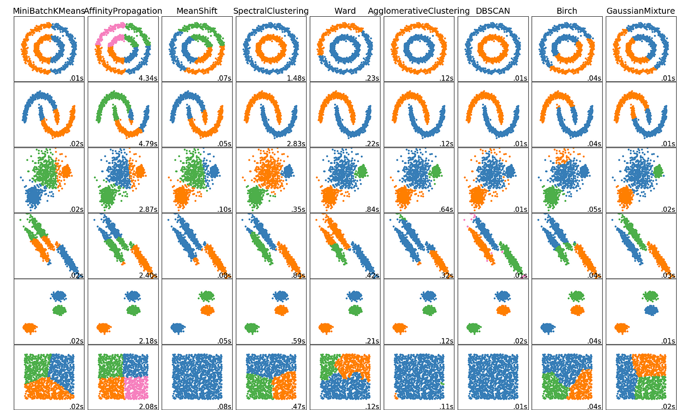
This image shows different kinds of clusters formed by different clustering algorithms. Out of these the project explores K-Means, Hierarchical and DBSCAN clustering techniques.
Distance metrics are fundamental to clustering algorithms as they define what "similarity" means in the context of the data. Euclidean distance, the most common metric, measures the straight-line distance between points in Euclidean space. Manhattan distance sums the absolute differences of coordinates, making it useful when features represent discrete steps. Cosine similarity measures the cosine of the angle between vectors, focusing on orientation rather than magnitude, which is particularly useful for high-dimensional data where the magnitude might be less important than the pattern of features.
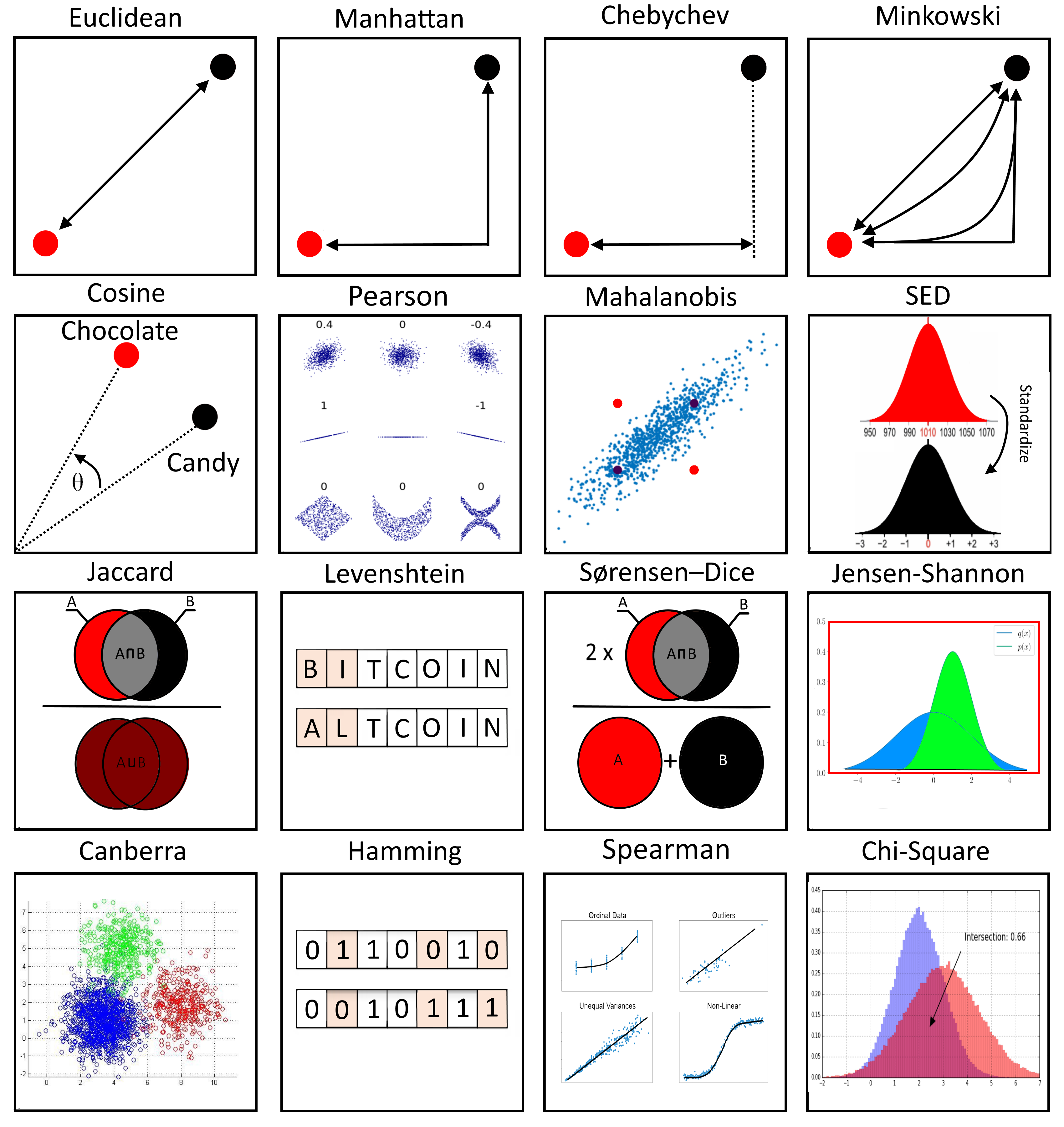
This visualization illustrates a variety of distance metrics used in clustering algorithms. Euclidean distance represents the straight-line distance between points, while Manhattan distance follows grid lines. Cosine similarity measures the angle between vectors, regardless of their magnitudes.
In the analysis of this audio dataset, the focus is on three prominent clustering algorithms: K-means, Hierarchical clustering, and DBSCAN (Density-Based Spatial Clustering of Applications with Noise). Each offers unique advantages for discovering patterns in the high-dimensional audio feature space.
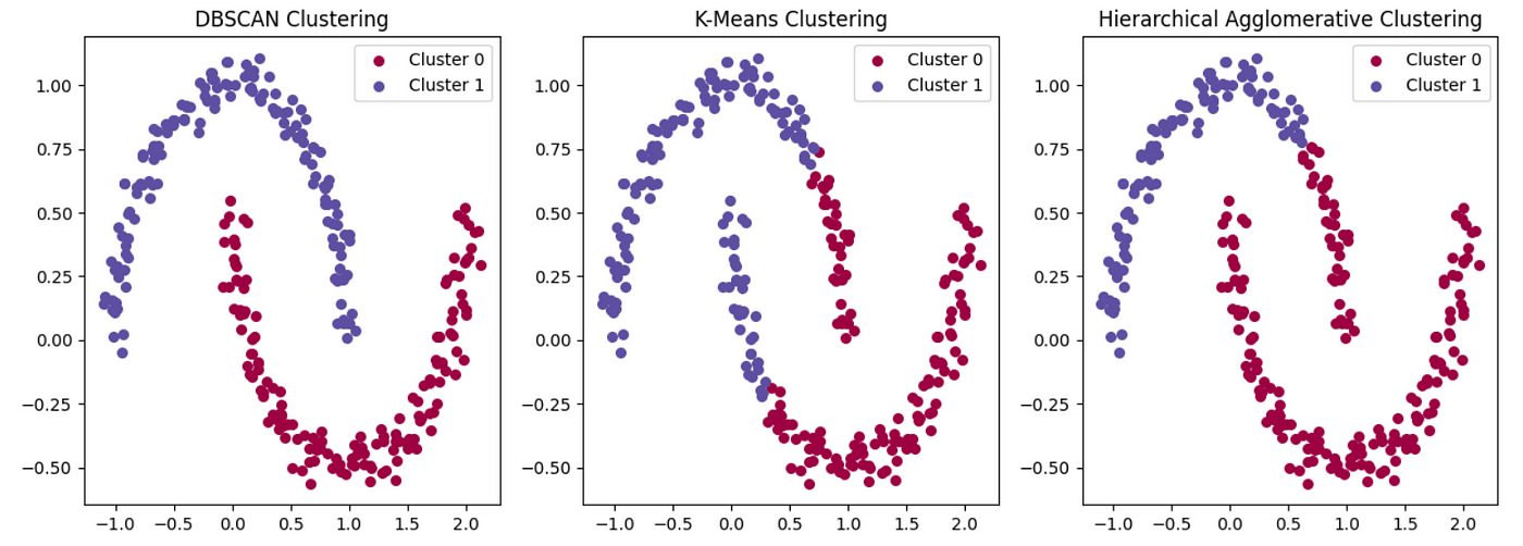
This comparison illustrates how the three clustering methods approach the same dataset differently. K-means (centre) partitions the space into Voronoi cells, with each point assigned to the nearest centroid. Hierarchical clustering (right) builds a tree-like structure of nested clusters. DBSCAN (left) identifies dense regions separated by sparser areas, capable of finding arbitrary-shaped clusters and identifying outliers. These difference in approaches lead to different formed clusters.
Comparing Clustering Approaches
K-Means Clustering
K-means is a partitioning method that divides data into K non-overlapping clusters by iteratively assigning points to the nearest centroid and updating centroids based on the mean of assigned points. It excels with spherical clusters of similar size and density but requires specifying the number of clusters beforehand and is sensitive to outliers and initial centroid placement.
Hierarchical Clustering
Hierarchical clustering builds a tree of nested clusters by either merging (agglomerative) or splitting (divisive) groups. It doesn't require pre-specifying the number of clusters and provides a dendrogram visualization of the clustering process. However, it can be computationally intensive for large datasets and requires choosing a linkage method (e.g., Ward's, complete, single) that defines how distances between clusters are measured.
DBSCAN
DBSCAN (Density-Based Spatial Clustering of Applications with Noise) identifies clusters as dense regions separated by sparser areas. It doesn't require specifying the number of clusters and can discover arbitrarily shaped clusters while identifying outliers as noise. However, it's sensitive to its parameters (epsilon and min_samples) and struggles with clusters of varying densities. DBSCAN is particularly useful for datasets with noise and non-spherical cluster shapes.
Preparing the Dataset for Clustering
For the clustering analysis, the 3D PCA-transformed dataset created in the previous section will be used. This approach offers two significant advantages: it reduces computational complexity by working with just three dimensions instead of the original 43, and it focuses on the most significant variance in the data, potentially leading to more meaningful clusters. The dataset maintains the category labels, allowing for evaluation of how well the clustering results align with the actual sound categories. Both the original dataset and the 3D PCA transformed datasets are shown below.
A preview of the original dataset showing the 43 acoustic features and category labels. Each row represents an audio sample, and each column represents a different acoustic feature. The second column as seen contains the sound category labels.
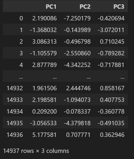
Preview of the PCA-transformed dataset used for clustering. Each row represents an audio sample with its three principal components. This reduced representation captures approximately 51% of the variance in the original feature space while making clustering analysis computationally tractable.
K-Means Clustering
The clustering analysis begins with K-means, one of the most widely used clustering algorithms. To determine the optimal number of clusters, the silhouette method was applied, which measures how similar objects are to their own cluster compared to other clusters. The silhouette score ranges from -1 to 1, with higher values indicating better-defined clusters.
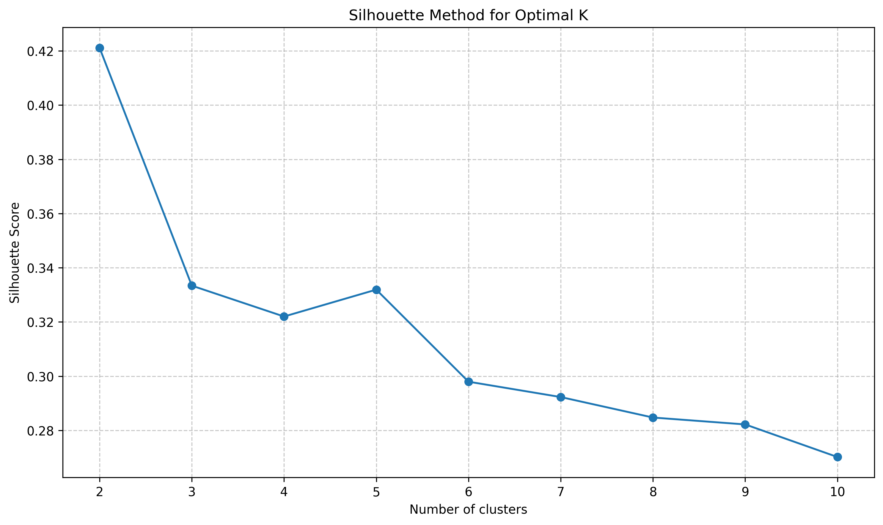
This plot shows the silhouette scores for different numbers of clusters (K values from 2 to 10). Based on this analysis, the highest silhouette scores were achieved with K=2, K=3, and K=5, suggesting these are the most natural groupings for the audio data when using K-means clustering.
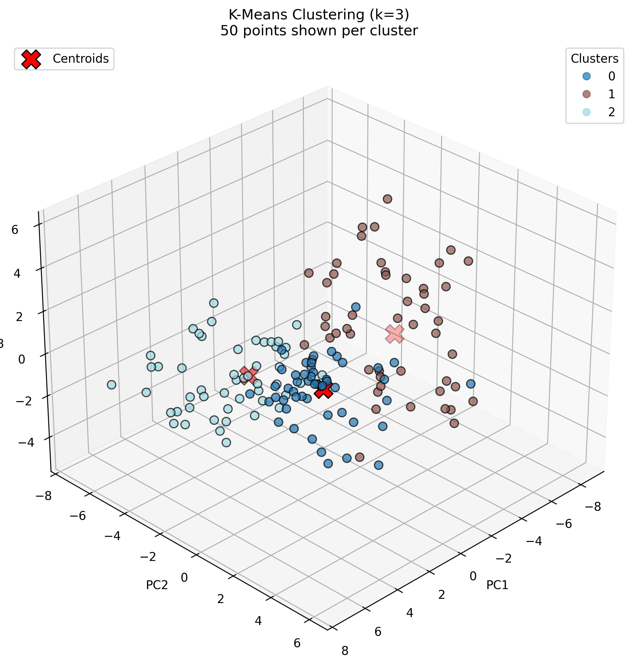
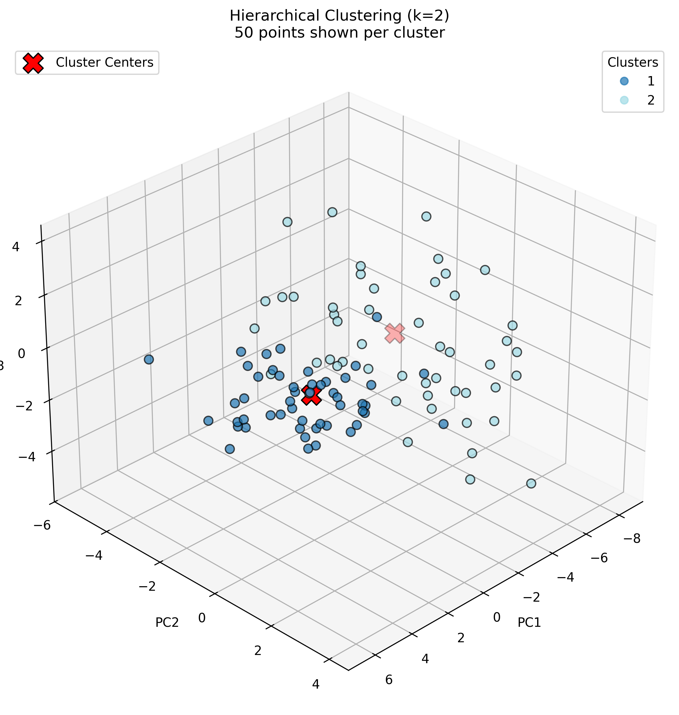
Based on the silhouette analysis, K-means clustering was performed with K=2, K=3, and K=5. For visualization clarity, 50 samples per sound category were randomly selected to create the 3D cluster plots.
K-Means with K=2
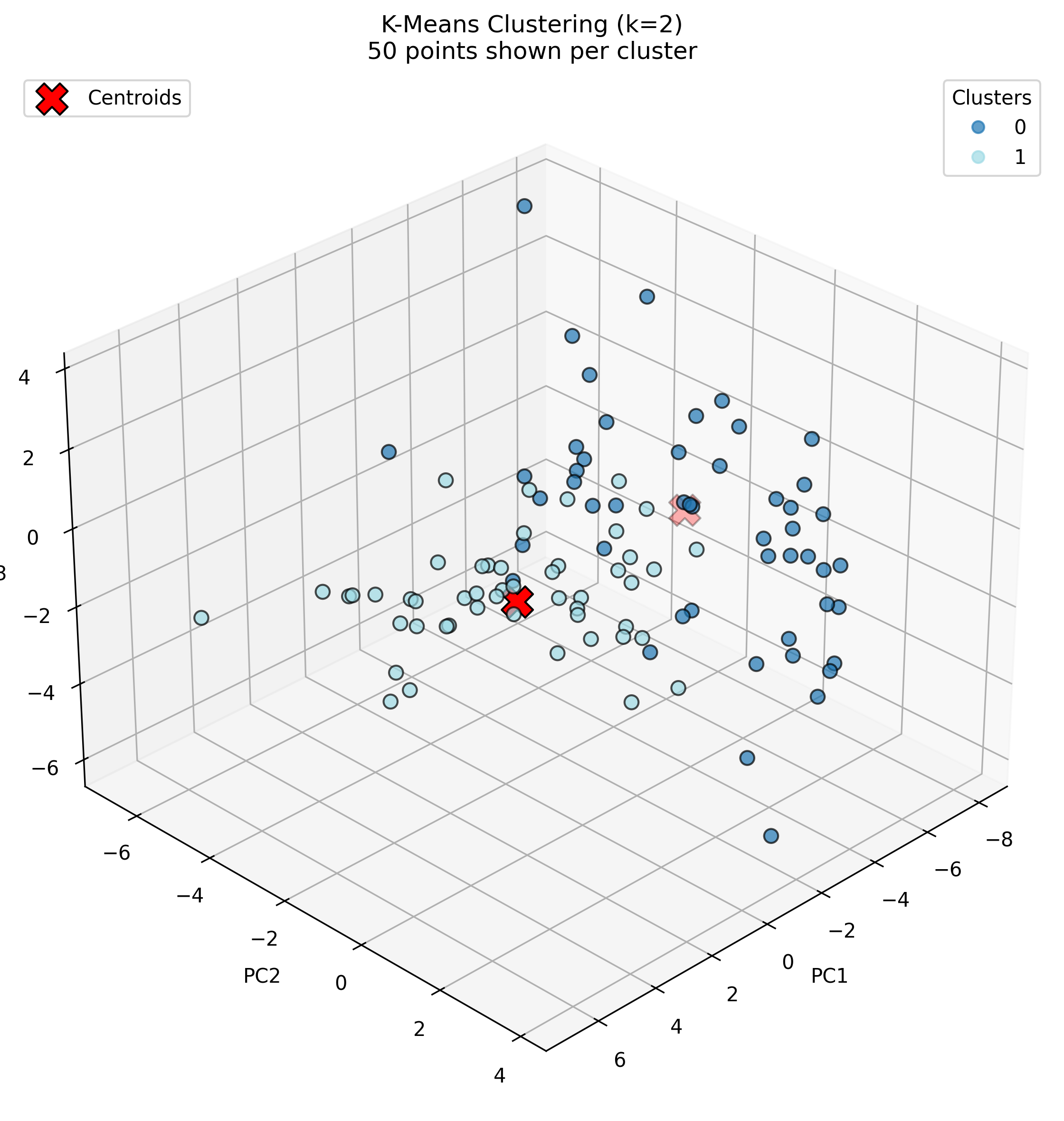
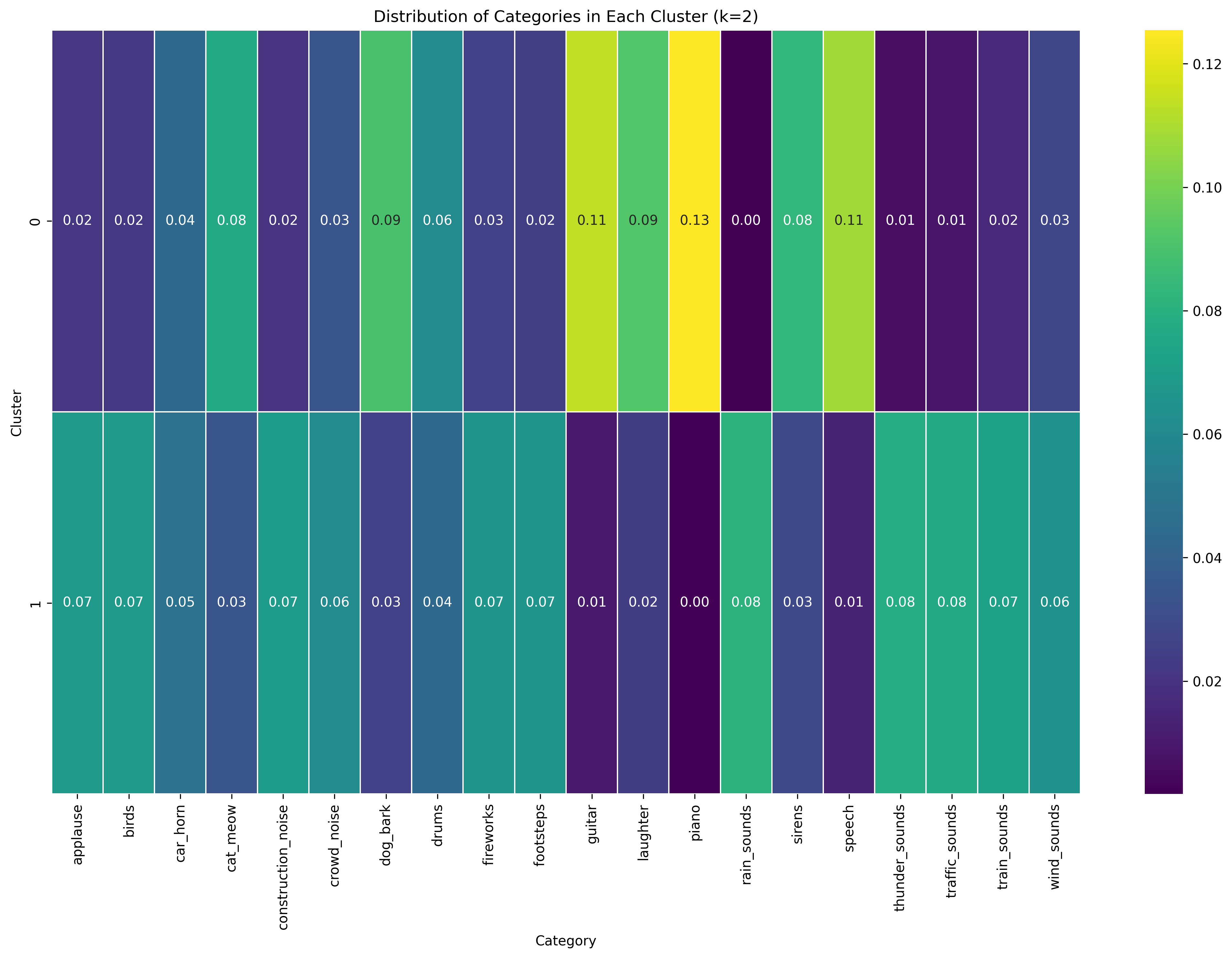
With K=2, the algorithm creates a clear distinction between two sound types. Cluster 0 shows high concentrations of piano (0.13), guitar (0.11), laughter (0.09), dog bark (0.09), and speech (0.11), suggesting it captures musical, vocal, and animal sounds. Cluster 1 displays more uniform distribution across categories with higher values for applause (0.07), birds (0.07), and various environmental sounds like thunder, traffic, and wind sounds, indicating it encompasses more ambient and environmental noise categories.
K-Means with K=3
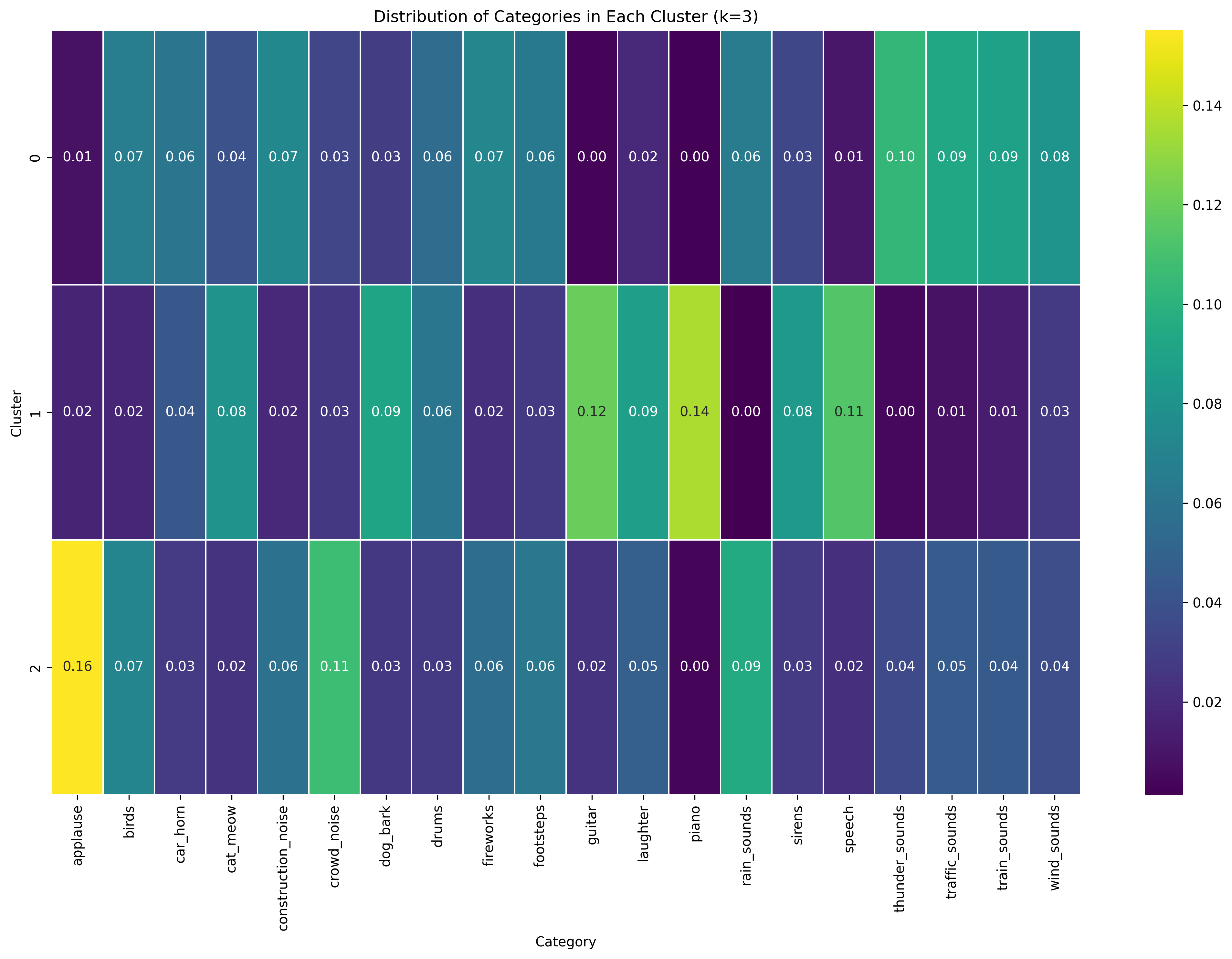
With K=3, the separation becomes more refined. Cluster 0 maintains a balanced distribution with higher values for thunder sounds (0.10), traffic sounds (0.09), and wind sounds (0.08). Cluster 1 shows peaks for guitar (0.12) and crowd noise (0.12), while Cluster 2 is strongly dominated by piano (0.14) and applause (0.16). This suggests a division between ambient sounds (Cluster 0), mixed social/instrumental sounds (Cluster 1), and percussion-heavy sounds with applause (Cluster 2).
K-Means with K=5
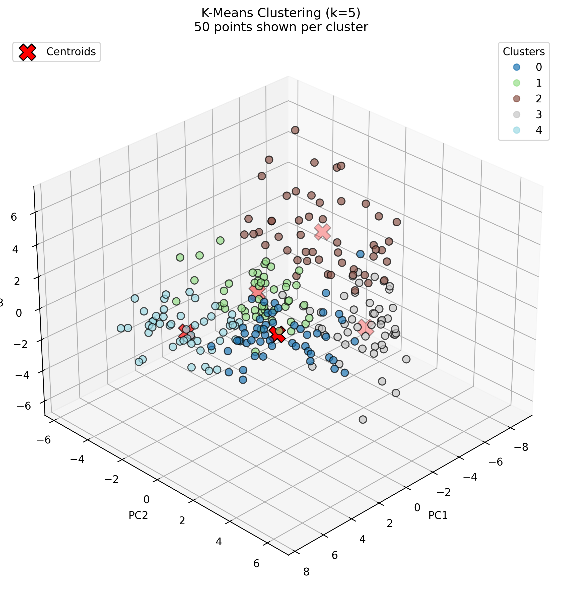
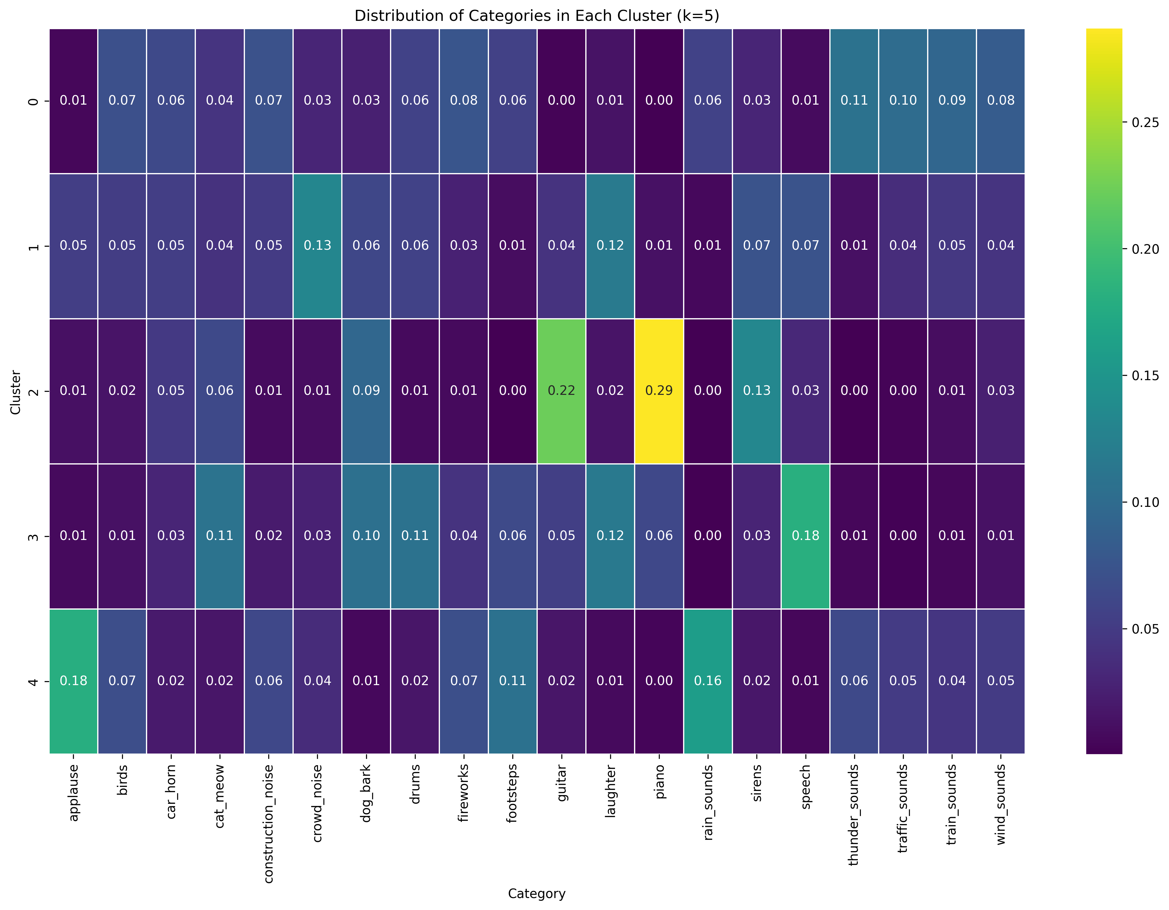
With K=5, the algorithm produces even more specialized clusters. Cluster 2 shows the strongest specialization with very high concentrations of piano (0.29) and guitar (0.22), clearly capturing musical instruments. Cluster 4 is characterized by applause (0.18) and rain sounds (0.16). Cluster 3 shows peaks for construction noise (0.11), drums (0.11), and speech (0.18), suggesting it captures percussive and vocal sounds. Clusters 0 and 1 appear to capture remaining environmental and mechanical sounds, with Cluster 0 showing higher values for various traffic and wind sounds, and Cluster 1 having a notable peak for crowd noise (0.13).
Hierarchical Clustering
Next, we applied hierarchical clustering using cosine similarity as our distance metric, which measures the angle between feature vectors rather than their Euclidean distance. This approach is particularly useful for exploring nested relationships between sound categories and for examining the clustering structure at different levels of granularity. Cosine similarity focuses on the orientation of vectors rather than their magnitude, making it well-suited for audio feature data where the pattern of spectral characteristics is often more important than their absolute values.
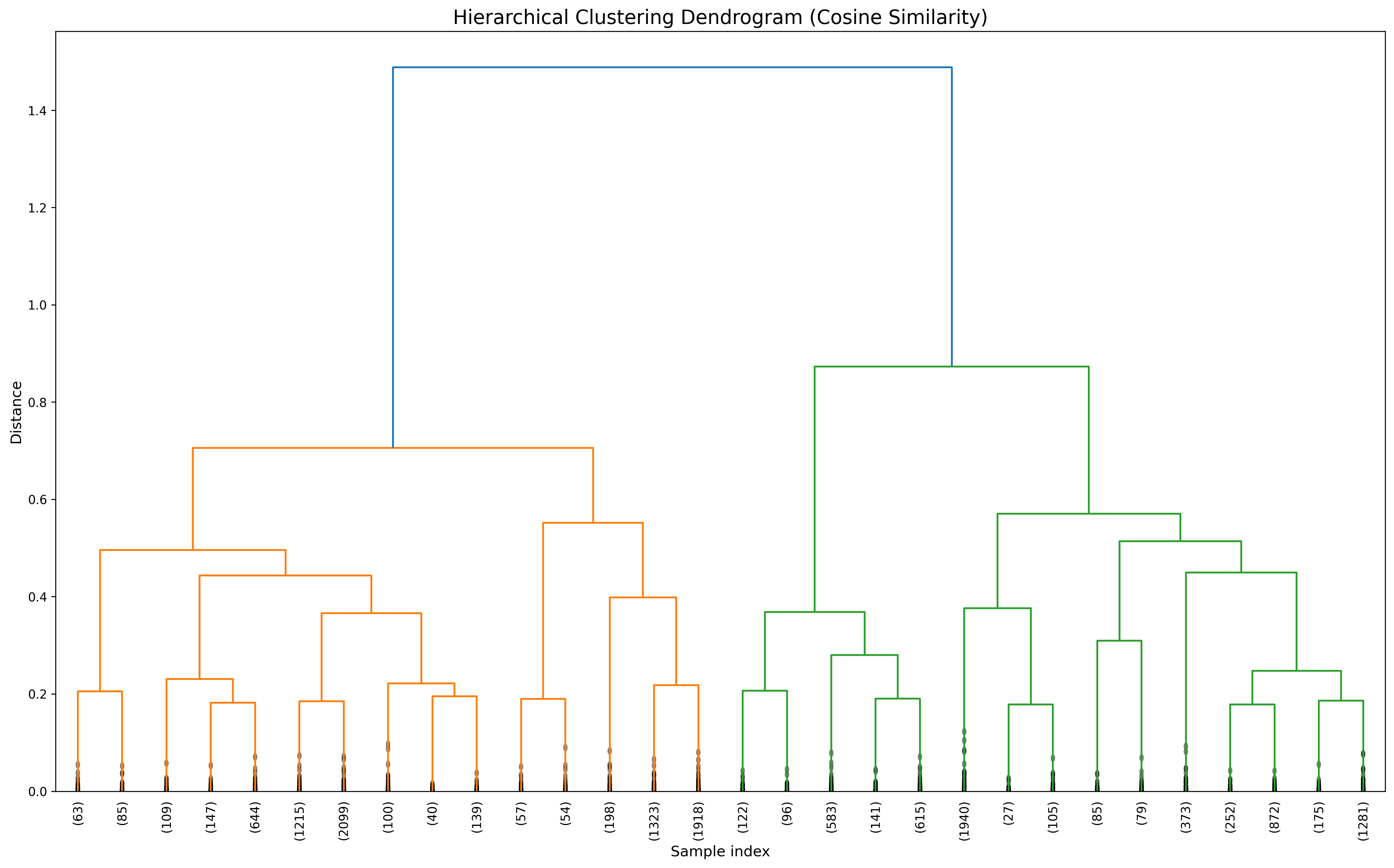
This dendrogram visualizes hierarchical relationships using cosine similarity as the distance metric. The plot reveals two primary clusters (orange and green) that diverge at a distance of about 1.5. The orange cluster contains several subclusters that merge at distances between 0.2-0.7, while the green cluster shows a different internal structure. By "cutting" the dendrogram at various heights, we can obtain different numbers of clusters to suit our analysis needs, providing flexibility in how we group the audio samples.
To compare with our K-means results, we "cut" the dendrogram to create 2, 3, and 5 clusters:
Hierarchical Clustering with 2 Clusters
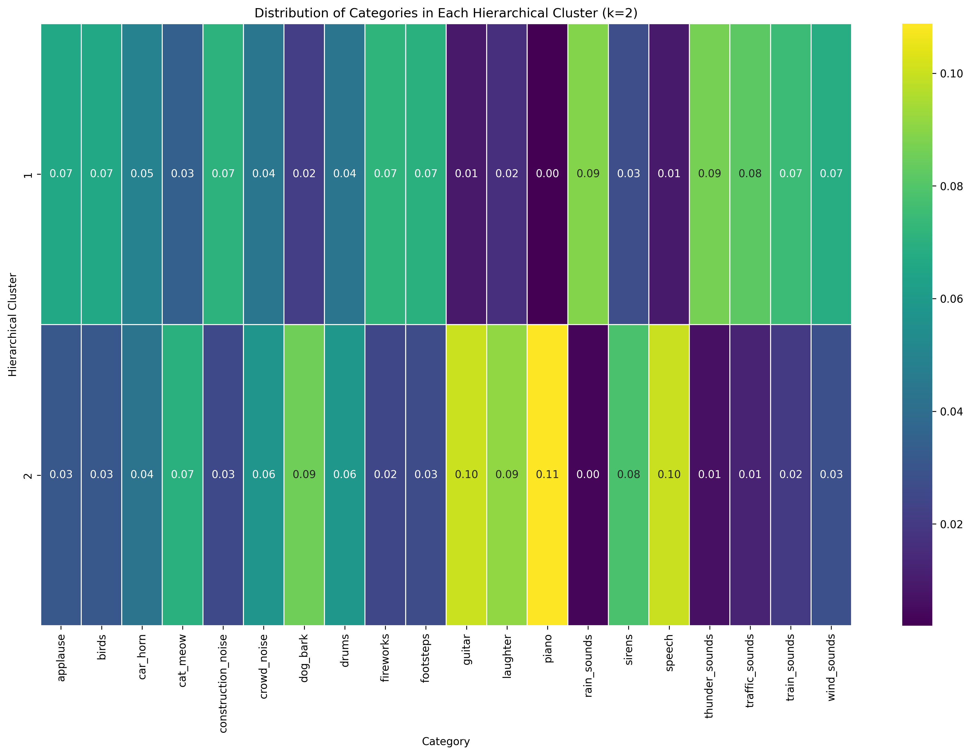
Looking at the k=2 hierarchical clustering solution (Image 3), a clear division exists between two types of audio. Cluster 1 shows a relatively even distribution across many sound categories with moderate values (0.07-0.09) for rain_sounds, thunder_sounds, applause, birds, and fireworks. Cluster 2 shows notably high concentrations for piano (0.11), guitar (0.10), laughter (0.09), and speech (0.10), suggesting this cluster primarily captures musical and human vocal sounds. The distribution pattern indicates a separation between musical/vocal sounds and environmental/ambient sounds.
Hierarchical Clustering with 3 Clusters
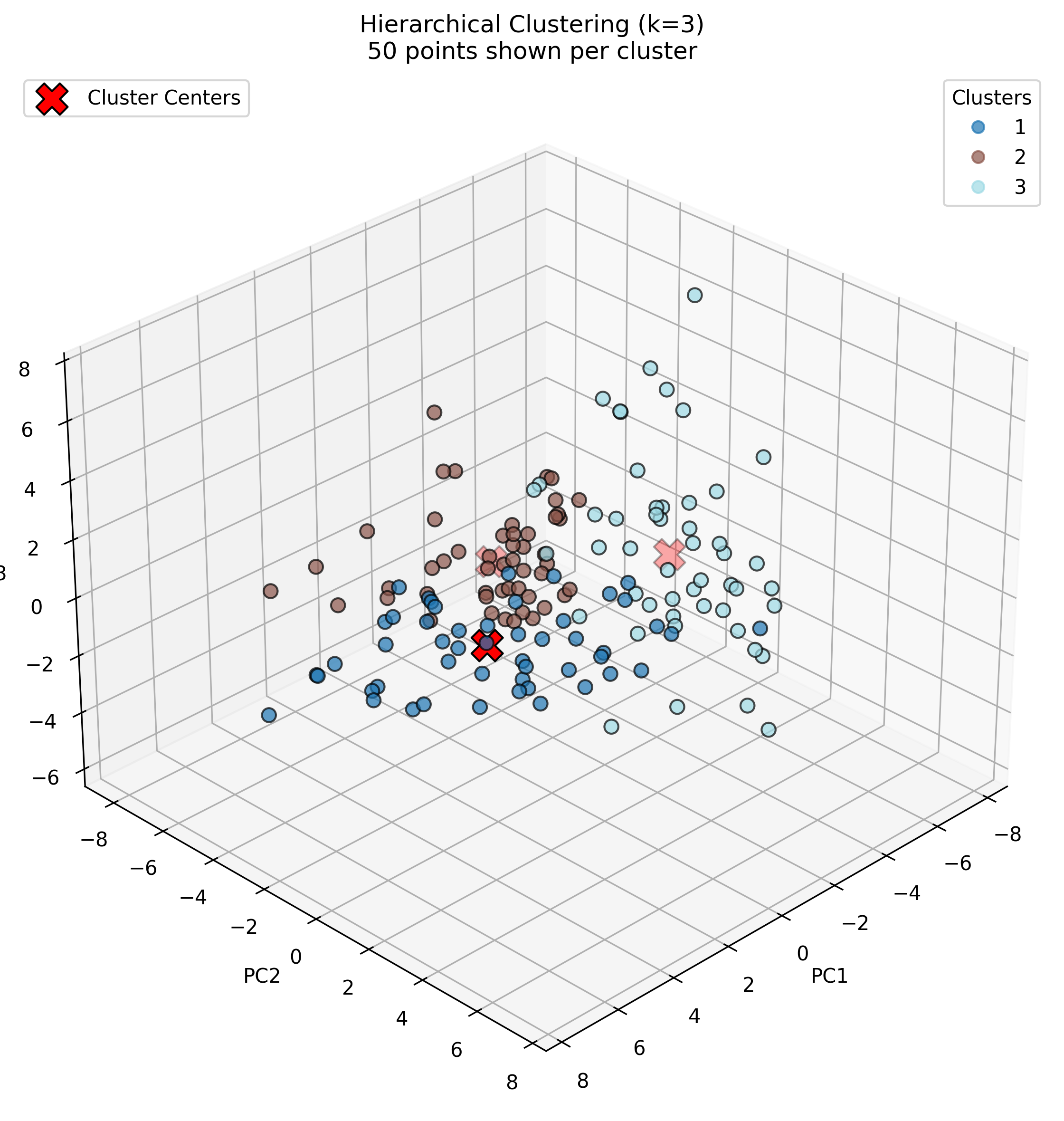
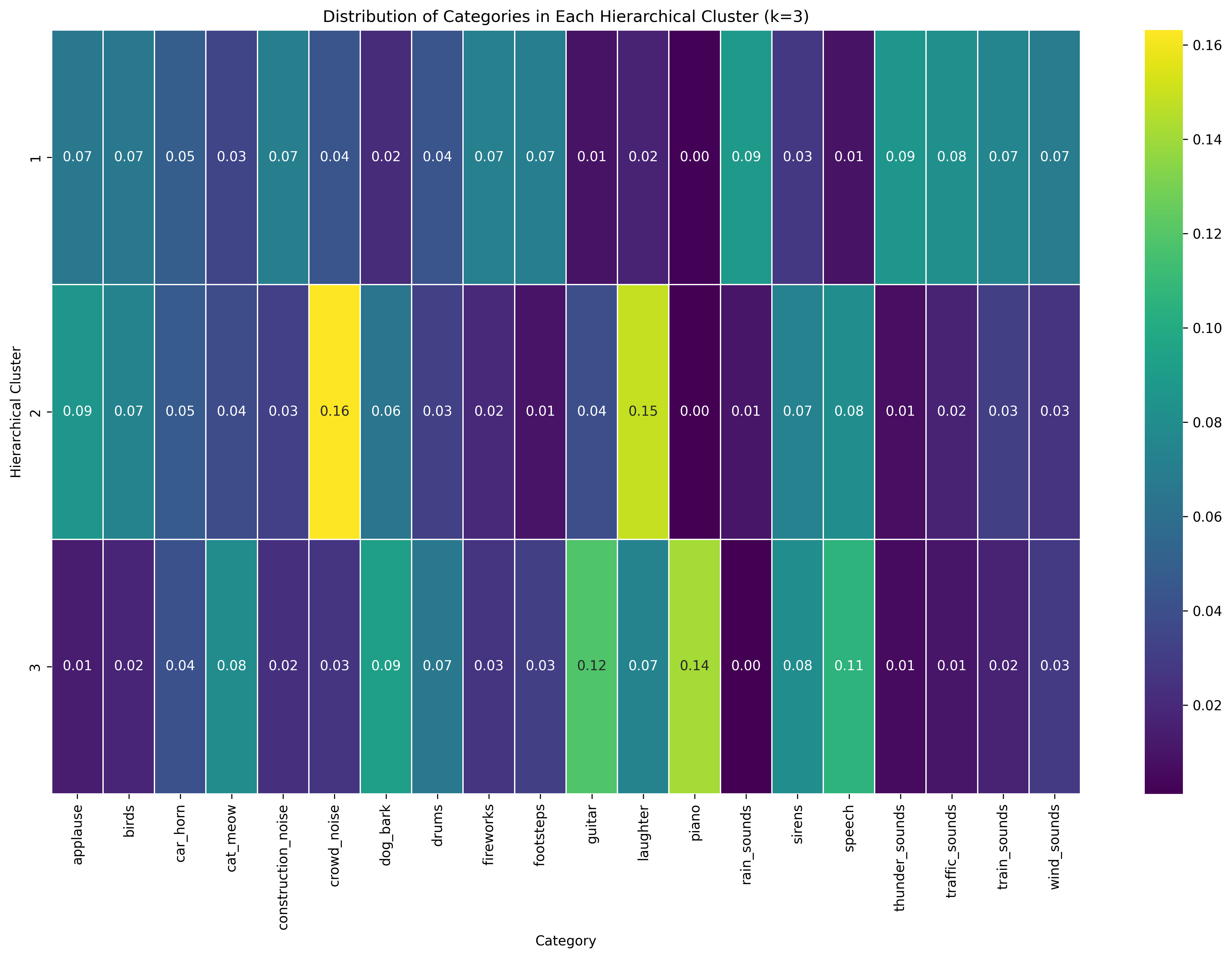
In the k=3 hierarchical clustering solution (Image 1), a more refined categorization emerges. Cluster 1 maintains relatively even distribution across categories with slightly higher values for thunder_sounds and train_sounds. Cluster 2 shows strong peaks for crowd_noise (0.16) and laughter (0.15), suggesting it captures human-generated ambient sounds. Cluster 3 has notable concentrations in laughter (0.14), guitar (0.12), and speech (0.11), indicating it primarily identifies musical and speech-related audio. This three-cluster solution provides better differentiation between natural environmental sounds, human ambient sounds, and musical/speech sounds.
Hierarchical Clustering with 5 Clusters
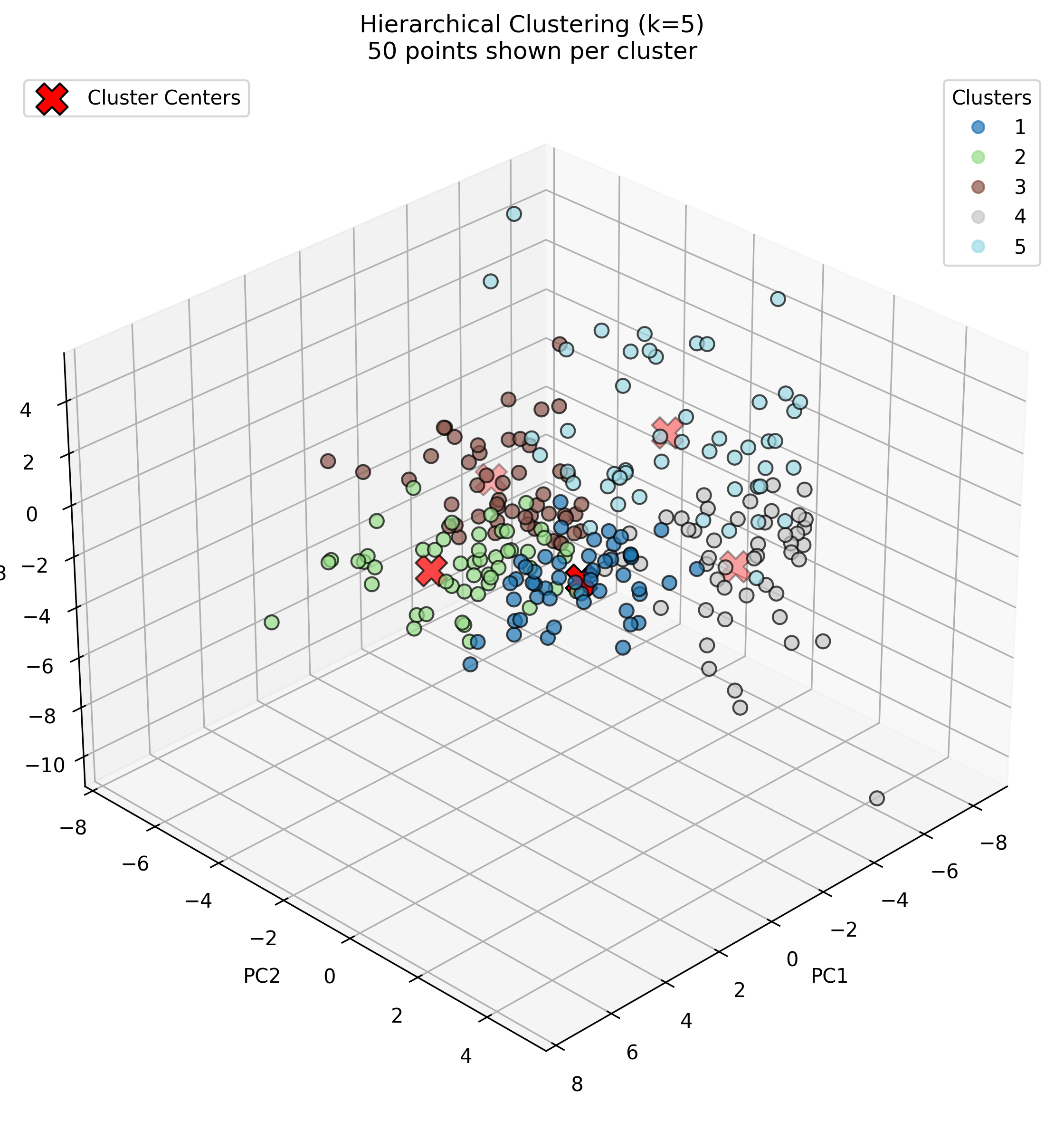
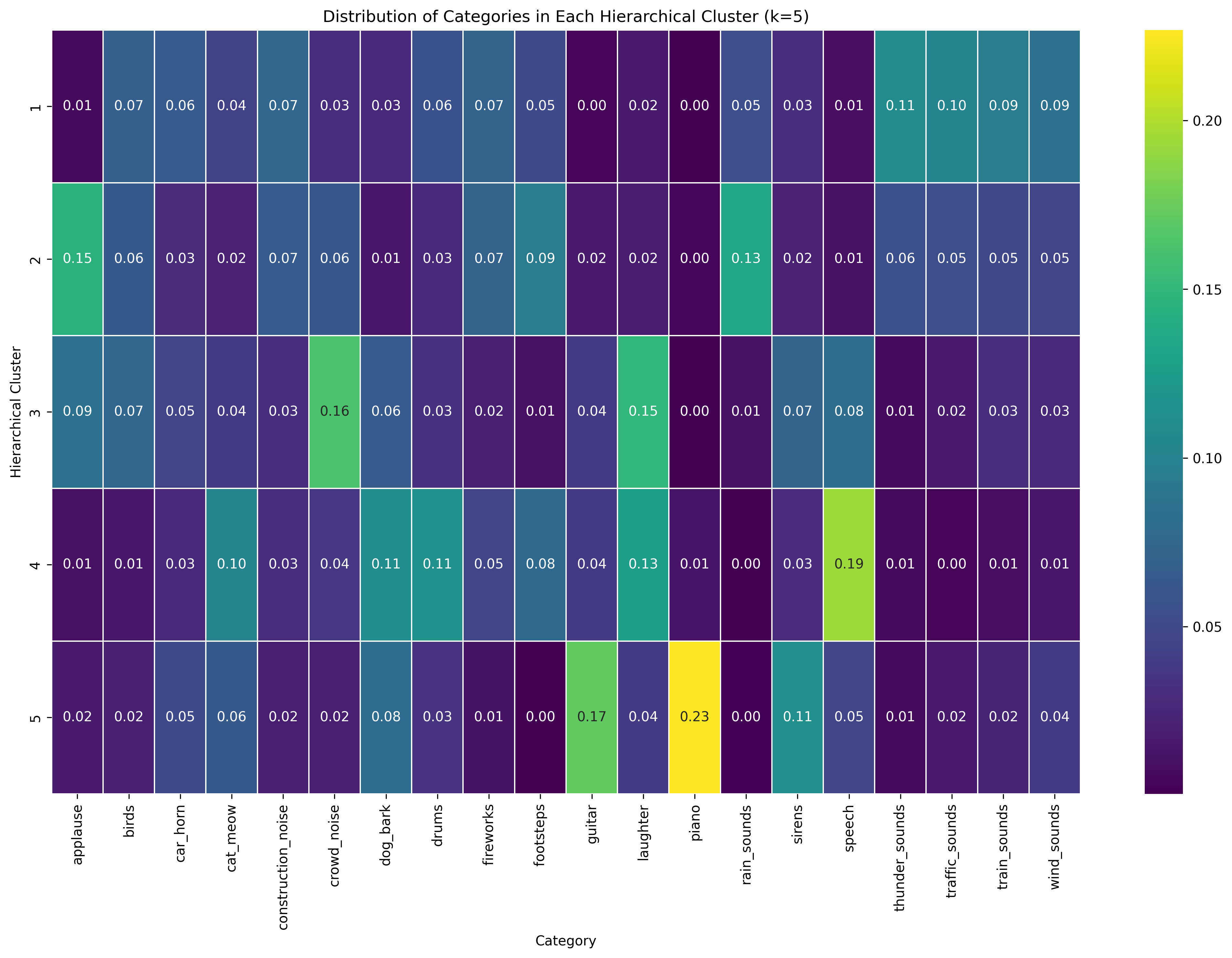
The k=5 hierarchical clustering solution (Image 2) offers the most granular categorization. Cluster 1 shows higher values for thunder_sounds (0.11), traffic_sounds (0.10), and train_sounds (0.09). Cluster 2 peaks at applause (0.15) and rain_sounds (0.13). Cluster 3 maintains the crowd_noise (0.16) and laughter (0.15) pattern. Cluster 4 distinctively peaks at speech (0.19), while Cluster 5 shows the highest concentration for piano (0.23) with a secondary peak at guitar (0.17). This five-cluster solution effectively separates environmental sounds (Clusters 1-2), human ambient sounds (Cluster 3), speech (Cluster 4), and musical instruments (Cluster 5), demonstrating how increasing k reveals more nuanced audio categorization patterns.
DBSCAN Clustering
DBSCAN was applied as the final clustering technique. This density-based algorithm identifies clusters without requiring pre-specified cluster numbers, unlike K-means and hierarchical clustering. DBSCAN automatically detects dense regions separated by sparser areas and can identify outliers as noise points, providing a different perspective on audio categorization.
The optimal epsilon (neighborhood radius) parameter was determined using the k-distance method. This approach plots the distance to the kth nearest neighbor for each point. A suitable epsilon value is indicated by the "knee" or "elbow" in this plot. Multiple epsilon values around this point were explored, along with various min_samples values, to identify the optimal DBSCAN configuration.
Based on parameter exploration, optimal values of epsilon (neighborhood radius) and min_samples (minimum points required to form a dense region) were identified. Using these parameters, DBSCAN produced the following clustering result:
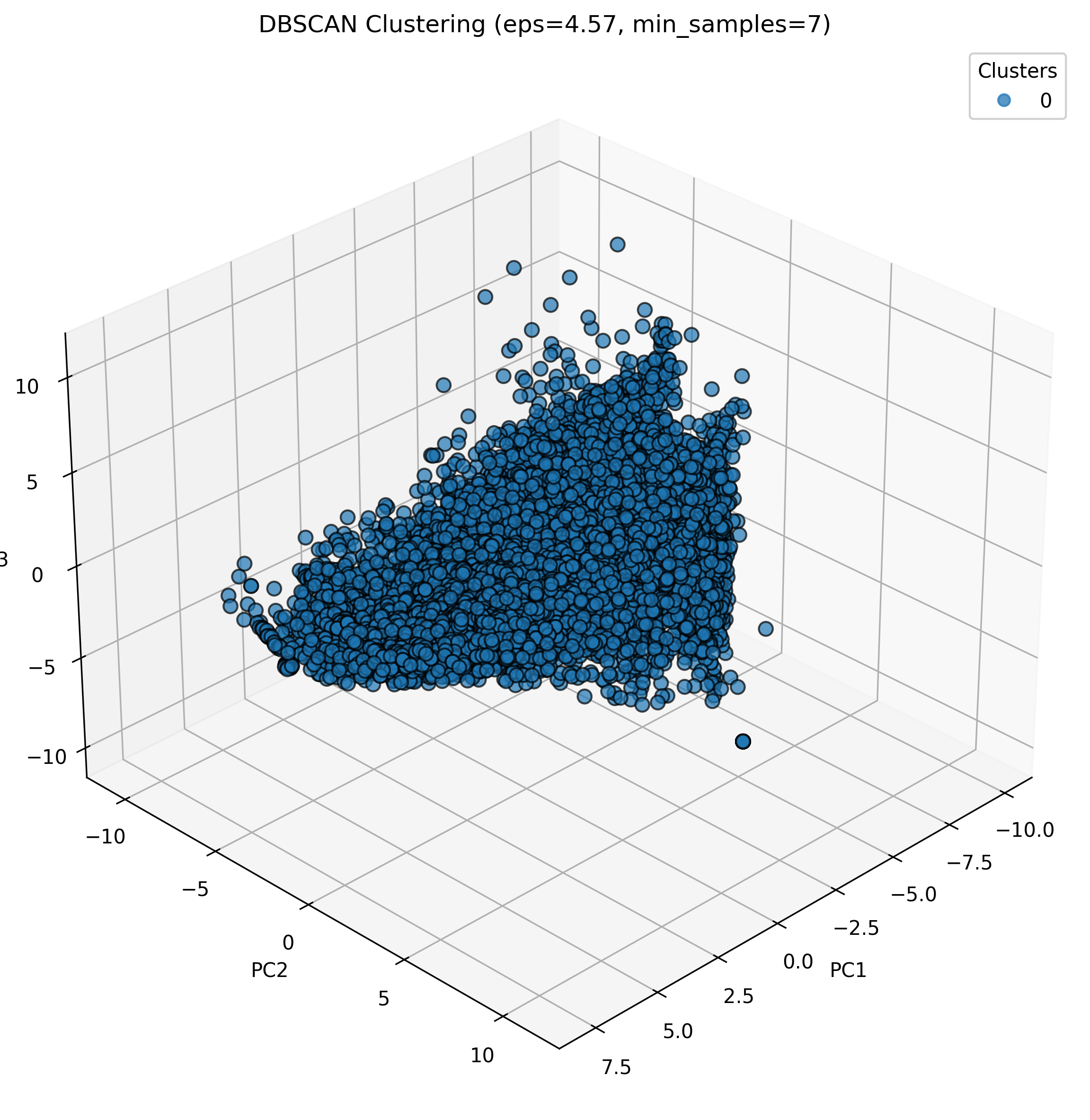
The DBSCAN clustering identified one major cluster containing all data points, with several points categorized as noise (shown in black). This result differs significantly from the K-means and hierarchical clustering results, suggesting that the audio data forms a continuous distribution in the PCA space rather than well-separated density-based clusters.
Clustering Comparison and Conclusion
The clustering analysis reveals interesting patterns in the audio dataset:
- K-means and hierarchical clustering both identify natural groupings that align with intuitive categories of sounds: musical instruments, speech and vocalizations, and environmental noises.
- Hierarchical clustering with Ward's linkage produces more compact and well-separated clusters than K-means, particularly for musical instruments.
- DBSCAN suggests that our audio data forms a continuous distribution rather than clearly separated density-based clusters in the PCA space.
- The optimal number of clusters appears to be between 3 and 5, significantly fewer than the 20 predefined sound categories, indicating natural acoustic similarities across different sound types.
In conclusion, this clustering analysis provides valuable insights into the natural organization of sound categories based on their acoustic properties. The results could inform the development of automatic sound classification systems by highlighting which categories are inherently similar and which are acoustically distinct. For instance, a hierarchical approach to classification might first distinguish between tonal and non-tonal sounds before making finer distinctions. Additionally, clustering helps explain why certain sound categories might be commonly confused in classification tasks, as they occupy similar regions in the acoustic feature space. These insights can guide feature engineering and model selection for supervised learning tasks in audio processing. The full script to perform clustering and the corresponding visualizations can be found here.
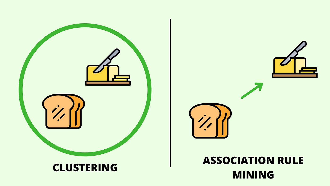
Association Rule Mining (ARM)
Association Rule Mining (ARM) is a technique used to discover interesting relationships between variables in large datasets. Unlike clustering, which groups similar items together, ARM identifies specific patterns of co-occurrence, answering questions like "What features frequently appear together?" or "If feature A has a high value, what can we predict about feature B?"
This diagram illustrates the concept of association rules. Rules take the form "If antecedent, then consequent" (A → B), indicating that when A occurs, B also tends to occur. In our audio analysis, this might be "If the zero-crossing rate is high and the spectral centroid is high, then the sound is likely a bird vocalization."
ARM uses several key metrics to evaluate the quality and usefulness of discovered rules:
- Support: The proportion of transactions (samples) that contain both the antecedent and consequent. Support measures how frequently a rule appears in the dataset.
- Confidence: The likelihood that the consequent occurs when the antecedent occurs. Confidence is calculated as the support of the entire rule divided by the support of the antecedent.
- Lift: A measure of how much more likely the consequent is when the antecedent occurs, compared to the consequent's overall frequency. Lift values greater than 1 indicate positive association, with higher values suggesting stronger relationships.
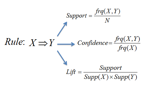
This image illustrates how support, confidence, and lift relate to each other. Support represents rule frequency, confidence shows prediction reliability, and lift indicates association strength. Strong rules have high values for all three metrics.
Apriori Algorithm
The Apriori algorithm is one of the most widely used methods for mining association rules. It works by first identifying frequent itemsets (sets of items that appear together frequently) and then generating rules from these itemsets. The algorithm uses a "bottom-up" approach, extending one item at a time and testing the frequency of each candidate itemset against a minimum support threshold.
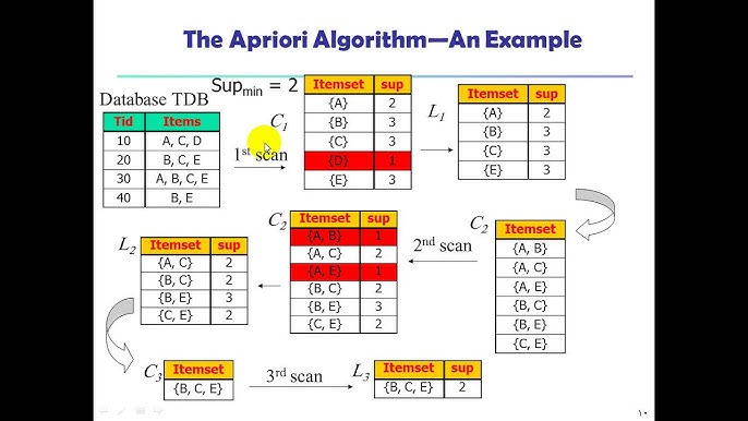
This image depicts an example of using Apriori algorithm.The visualization shows the process of discovering frequent itemsets and identifying meaningful associations between items in a dataset.
In audio analysis, Association Rule Mining (ARM) can reveal which acoustic features tend to co-occur and how they relate to sound categories. For instance, ARM can discover that specific combinations of spectral and temporal features strongly associate with particular sound types, providing interpretable insights into what makes different sounds acoustically distinctive.
Data Preparation for Association Rule Mining
ARM traditionally works with binary or categorical data, where items either appear in a transaction or don't. The audio dataset, however, contains continuous numerical features. To apply ARM, these continuous values needed to be transformed into categorical bins. The original dataset looks like this:
A representative subset of data was selected, comprising 100 samples from each of the 20 sound categories for a total of 2,000 samples. From the original 43 features, 15 key acoustic features were selected based on their importance in the PCA analysis:
- MFCC features (mfcc_1, mfcc_2, mfcc_4)
- Chroma features (chroma_3, chroma_7)
- Spectral contrast features (spectral_contrast_1, spectral_contrast_3)
- Basic audio descriptors (zero_crossing_rate, spectral_centroid, spectral_bandwidth, rms_energy, spectral_rolloff)
- Tonal features (tonnetz_1, tonnetz_3, tonnetz_6)
To discretize these continuous features, a simple but effective three-bin strategy was applied:
- Values below the 33rd percentile were labeled as "low"
- Values between the 33rd and 67th percentiles were labeled as "medium"
- Values above the 67th percentile were labeled as "high"
This transformation converted continuous features into categorical features suitable for ARM analysis. The transformed dataset is shown below:
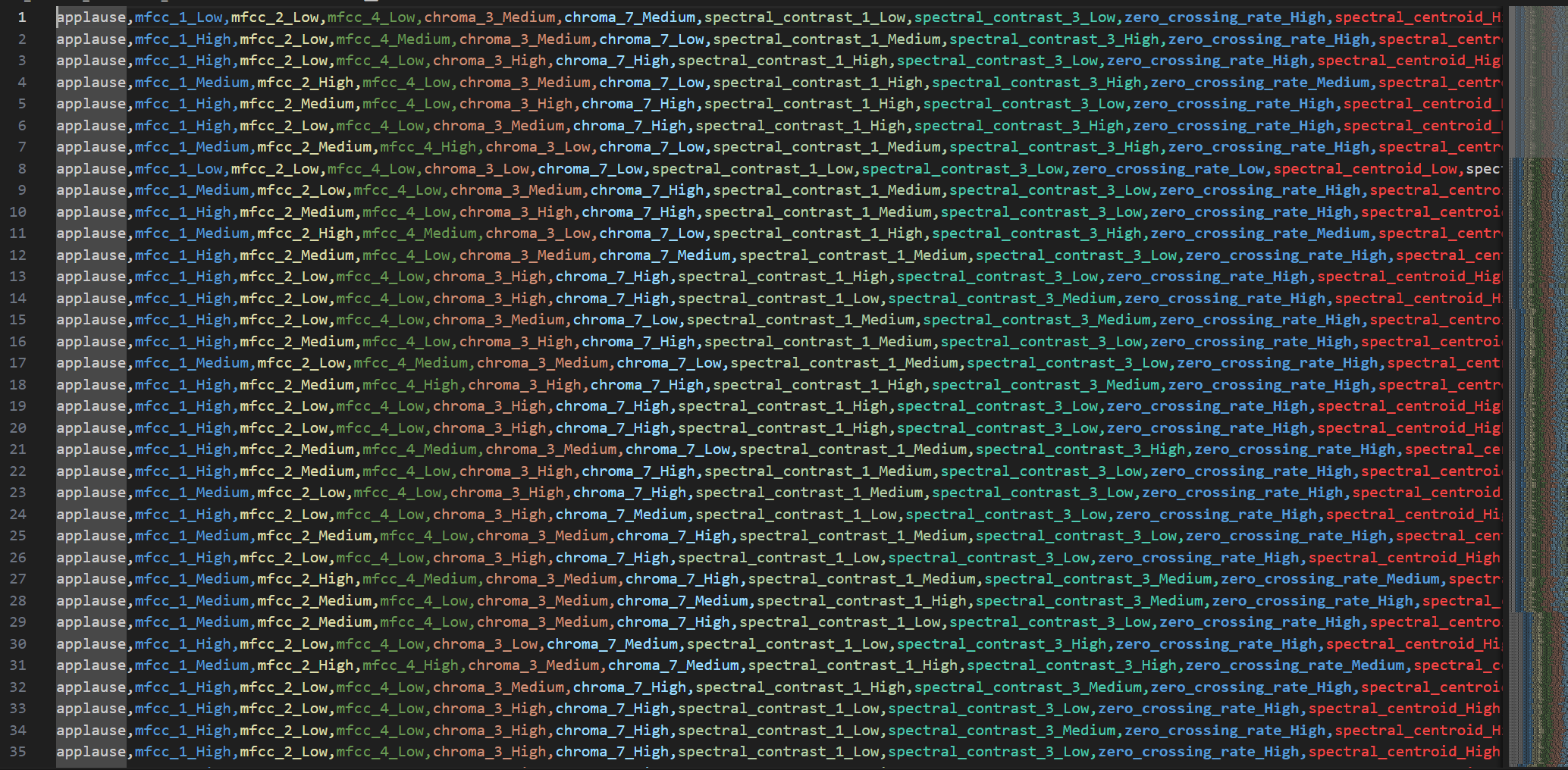
A preview of the transformed dataset after discretization. Each row represents an audio sample, and each column shows a feature's categorical value (low, medium, high) along with the sound category. This format allows for discovery of meaningful associations between feature ranges and sound types.
Applying Apriori Algorithm
The discretized dataset was used to apply the Apriori algorithm for discovering association rules. A minimum support threshold of 0.1 was set (meaning the rule must appear in at least 10% of the samples) and a minimum confidence threshold of 0.7 (meaning the rule must be correct at least 70% of the time).
After generating all rules that met these thresholds, the results were sorted by support, confidence, and lift to identify the most interesting and powerful associations.
Top 15 Rules by Support
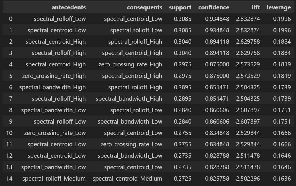
These rules have the highest support, meaning they appear most frequently in the dataset. High-support rules often represent common patterns but may not always provide the most distinctive insights.
Top 15 Rules by Confidence
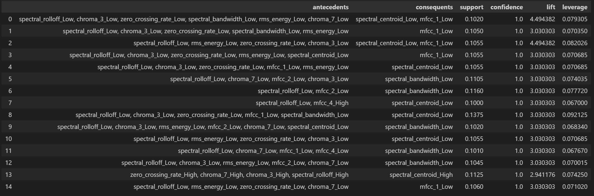
Rules with high confidence are highly reliable predictors. When the antecedent occurs, the consequent follows with high probability. These rules reveal that certain feature combinations can strongly predict other acoustic properties.
Top 15 Rules by Lift
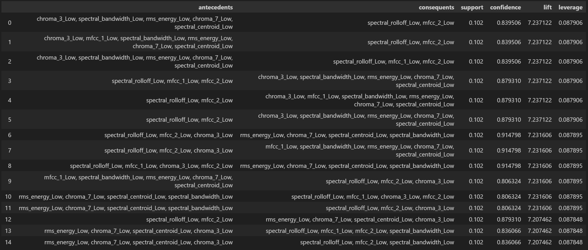
Lift measures how much more likely the consequent is when the antecedent occurs compared to its baseline probability. High-lift rules identify the strongest associations in our data, revealing distinctive acoustic signatures for different sound categories. These rules are particularly valuable for understanding what makes each sound type unique.
Association Network Visualization
The network visualization presents the strongest association rules discovered through ARM. Features and categories appear as nodes, while associations between them are displayed as edges. Edge thickness corresponds to rule lift, with thicker lines indicating stronger associations.
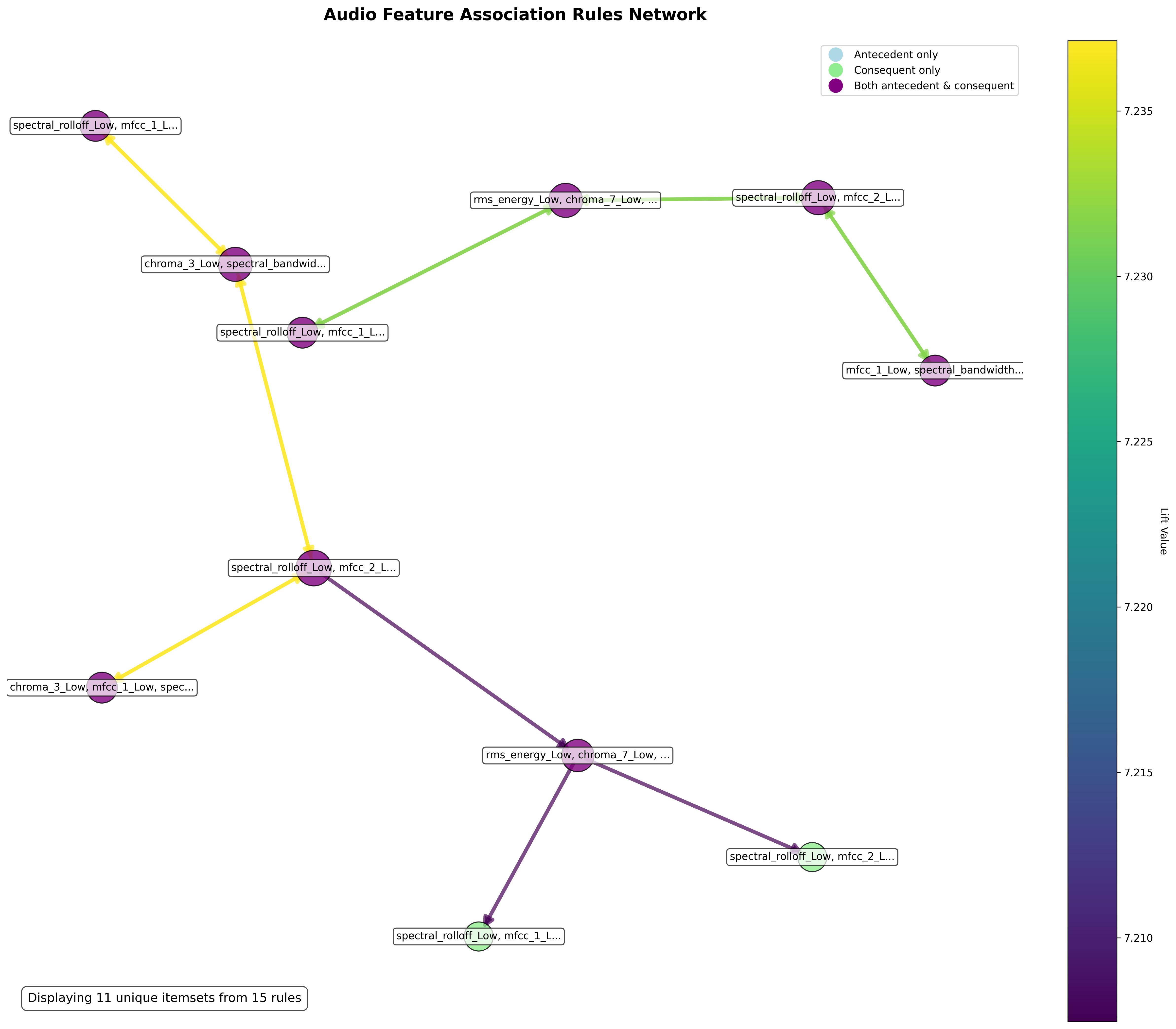
The network visualization reveals feature association patterns characterizing audio properties. Low spectral rolloff frequently appears with low MFCC values across multiple nodes, forming interconnected relationships. Several distinct pathways connect through RMS energy and chroma features, shown by the purple and yellow edges with varying strengths. The graph displays 11 unique itemsets derived from 15 rules, highlighting the most significant audio feature relationships in the analyzed dataset.
Conclusion
Association Rule Mining provided valuable insights into acoustic feature relationships. The discovered rules reveal strong connections between spectral features across different audio characteristics. For example, the top rules show that spectral_rolloff_Low strongly correlates with spectral_centroid_Low (support: 0.3085, confidence: 0.934848, lift: 2.832874), and similarly for their High value counterparts.
The more complex rules in the second and third tables demonstrate how combinations of low spectral features frequently appear together. Rules with perfect confidence (1.0) indicate that certain feature combinations invariably predict others, such as when multiple low spectral features (spectral_rolloff_Low, chroma_3_Low, etc.) consistently predict spectral_centroid_Low or mfcc_1_Low.
The highest lift values appear in the third table (approximately 7.23), indicating particularly strong associations between combinations of low spectral and chroma features. These patterns represent distinctive acoustic signatures that could characterize specific sound categories.
These association rules provide an interpretable understanding of acoustic feature relationships, complementing other analytical approaches. The knowledge gained has practical applications in sound recognition, audio classification, and can inform feature selection for supervised learning models by highlighting which acoustic properties show the strongest associations.
The full script to perform ARM and its corresponding visualizations can be found here.