Supervised Learning
Supervised learning is a cornerstone of machine learning where models learn from labeled training data to make predictions on unseen data. This section explores four powerful supervised techniques applied to the audio dataset: Naive Bayes for probabilistic classification, Decision Trees for rule-based decisions, Regression for predicting continuous values, and Support Vector Machines (SVM) for finding optimal decision boundaries. Each method offers unique strengths for audio classification tasks.
Naive Bayes
Overview
Naive Bayes is a family of probabilistic classifiers based on applying Bayes' theorem with a "naive" assumption that features are conditionally independent given the class. Despite this simplifying assumption, Naive Bayes classifiers often perform surprisingly well in practice, especially for text classification, spam filtering, sentiment analysis, and recommendation systems. They require relatively small amounts of training data to estimate the necessary parameters, train quickly, and are particularly suited to high-dimensional data. Naive Bayes models calculate the probability of each class given the feature values, selecting the class with the highest probability as the prediction.
The core idea is to flip the problem using Bayes' Theorem: instead of modeling the probability of features given a class being true (which can be hard), Naive Bayes models the likelihood of a class given the features. This makes it incredibly efficient, especially when combined with vectorized feature representations. Even when the independence assumption doesn't strictly hold, the model still tends to perform well in practice — a phenomenon sometimes called the "Naive Bayes miracle".
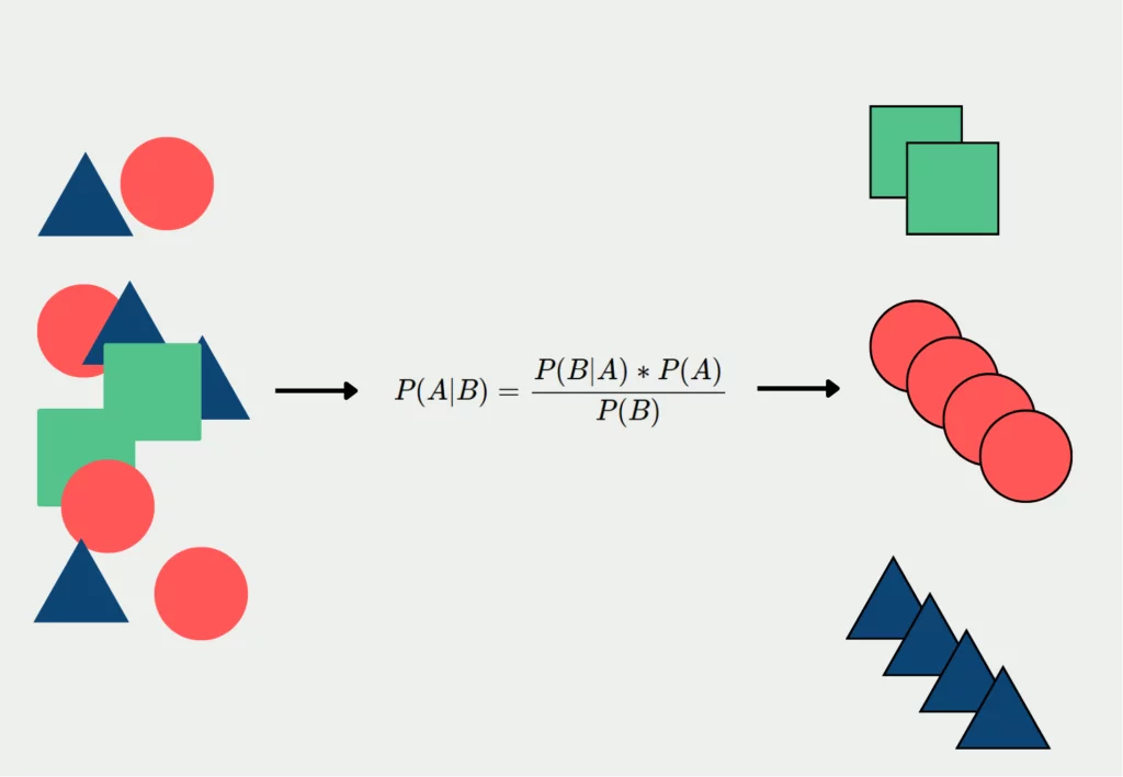
This diagram illustrates the fundamental concept of Naive Bayes classification. The model calculates the probability of each class based on observed features, making the "naive" assumption that features are conditionally independent given the class. This simplification allows for efficient computation even with many features.
Smoothing in Naive Bayes
One challenge with Naive Bayes is handling zero probabilities when a feature value doesn't appear in the training data for a given class. This can lead to the entire probability estimate for that class becoming zero due to multiplication. To address this, smoothing techniques like Laplace smoothing are used. These methods add a small constant to observed counts, ensuring that no probability is ever exactly zero. Smoothing helps improve generalization and ensures that the model can make predictions even for previously unseen feature values.
Without smoothing, even a single missing word or unseen feature could dominate the entire prediction, which can be disastrous in real-world applications. Laplace (add-one) smoothing or Lidstone (add-α) smoothing are common techniques that mitigate this, especially in domains like text classification where many features are sparse.
Different Types of Naive Bayes Classifiers
Naive Bayes' strength lies in its simplicity, computational efficiency, and effectiveness in many real-world scenarios. It excels when the independence assumption approximately holds or when the exact probability estimates are less important than the class rankings they produce. Different variants of Naive Bayes are suitable for different types of data:
Multinomial Naive Bayes
Suited for discrete counts, such as word frequencies in text classification. Features represent the frequencies with which certain events occur. Commonly used for document classification and spam filtering where feature vectors represent term frequencies.
Gaussian Naive Bayes
Appropriate for continuous data where features follow a normal distribution. Each class is modeled with a Gaussian distribution defined by mean and variance. Effective for classifying measurements like height, weight, or audio spectral features.
Bernoulli Naive Bayes
Designed for binary/boolean features. Models presence or absence of features rather than frequencies. Useful for text classification with binary word occurrence (present/absent) rather than counts, and in some cases of spam detection.
Categorical Naive Bayes
Handles categorical features directly without converting to numeric values. Each feature has its own categorical distribution per class. Particularly useful for nominal data where features have discrete, non-ordered categories.
The main differences between these variants lie in their assumptions about feature distributions. Multinomial assumes features follow a multinomial distribution suitable for count data. Gaussian works with continuous values assuming normal distributions. Bernoulli is optimal for binary features. Categorical handles nominal features without forcing numeric conversion. The appropriate variant should be selected based on the data characteristics for best performance.
Naive Bayes Classification of Audio Data
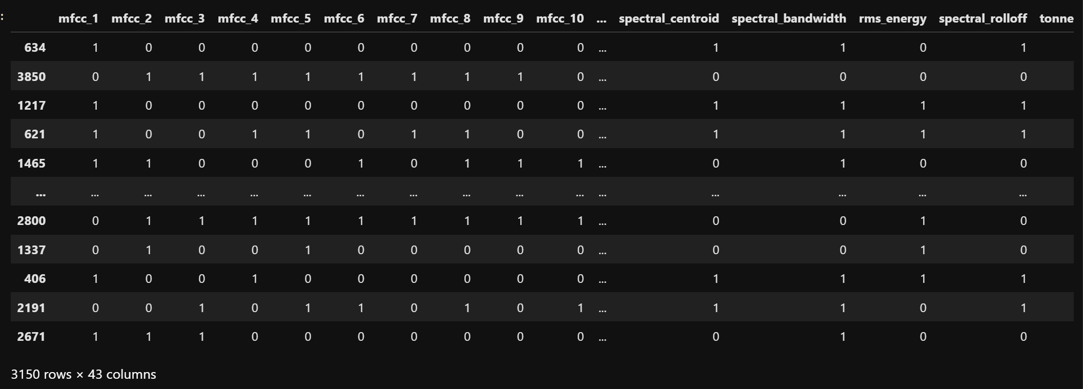
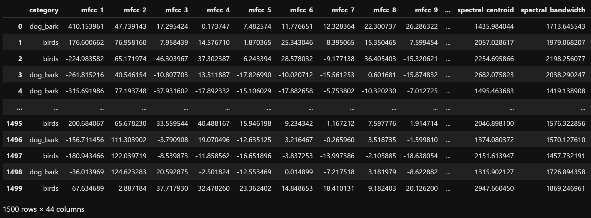
To apply Naive Bayes classification to audio data, a dataset consisting of extracted features from six sound categories: piano, guitar, drums, thunder sounds, rain sounds, and wind sounds, is selected. This dataset is shown below.
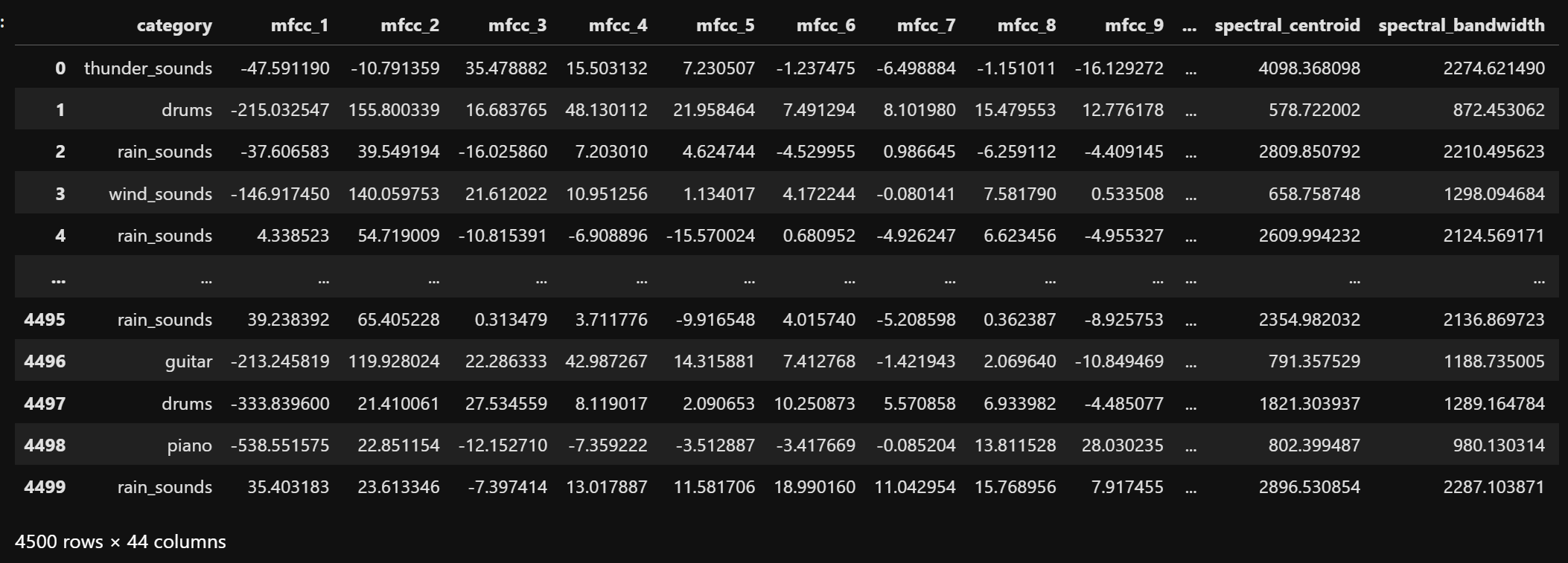
The dataset contains all the numeric audio features such as MFCCs, chroma, spectral contrast, tonnetz, and others, extracted for each audio file.
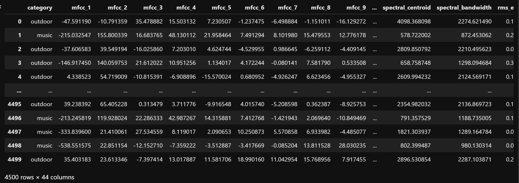
The raw data is grouped into two classes: music for records of categories piano, guitar, drums and outdoor for records of categories thunder, rain, wind. This transformation helps in converting a multi-class problem into a binary classification task, simplifying model training and evaluation. The categorized dataset is shown below.
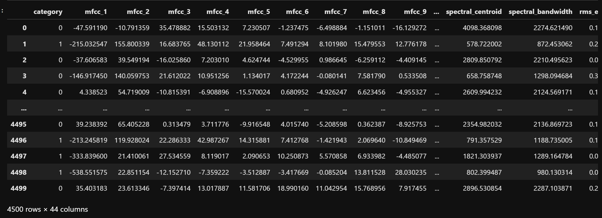
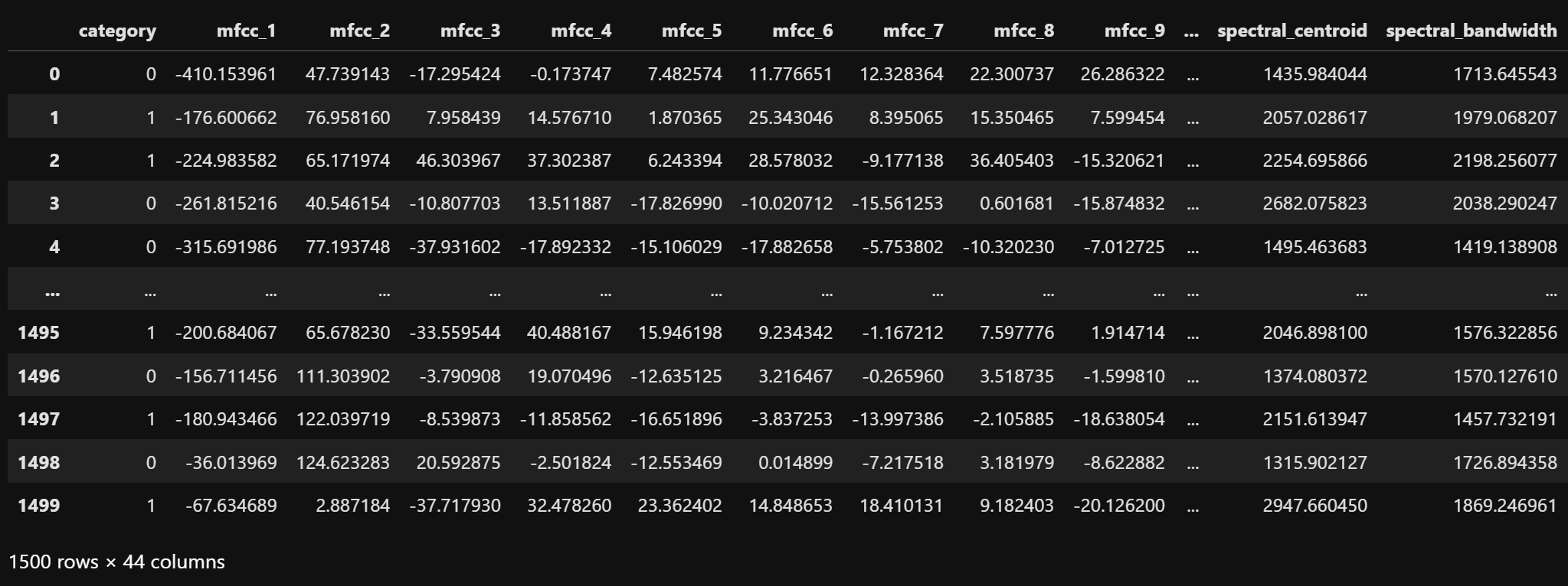
After categorization, the label column is encoded into binary form: music = 1 and outdoor = 0. This becomes the target variable for all the naive bayes classification models. The dataset after this transformation is shown below.
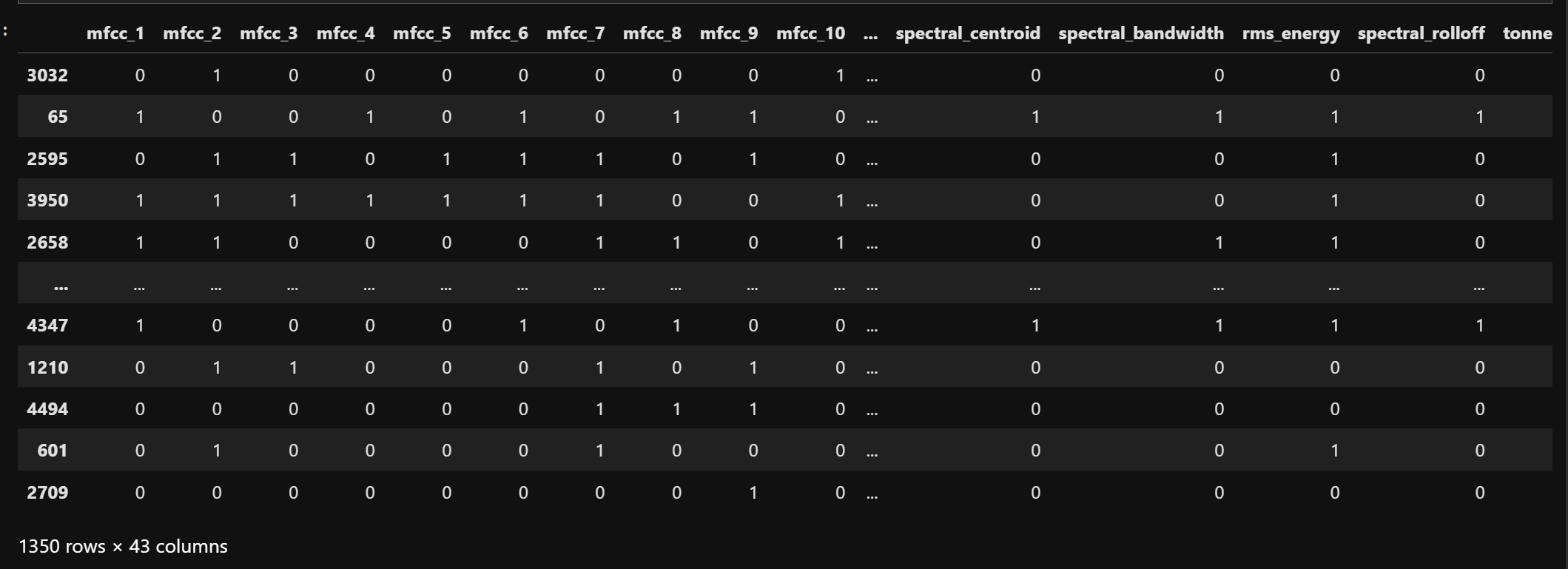
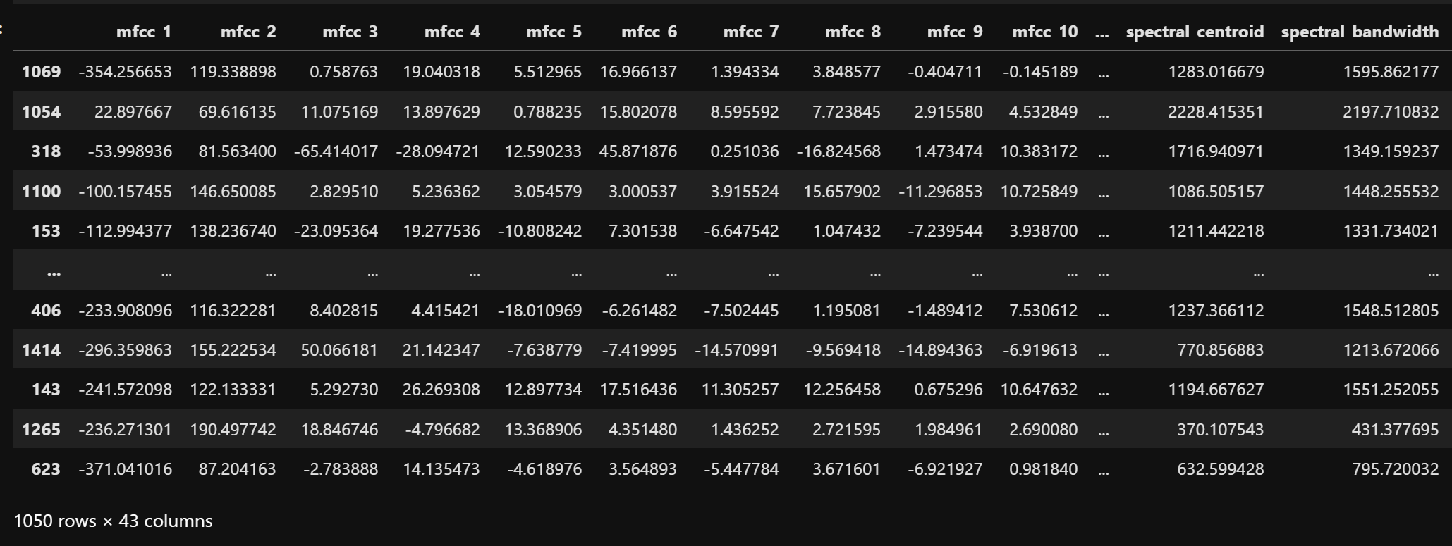
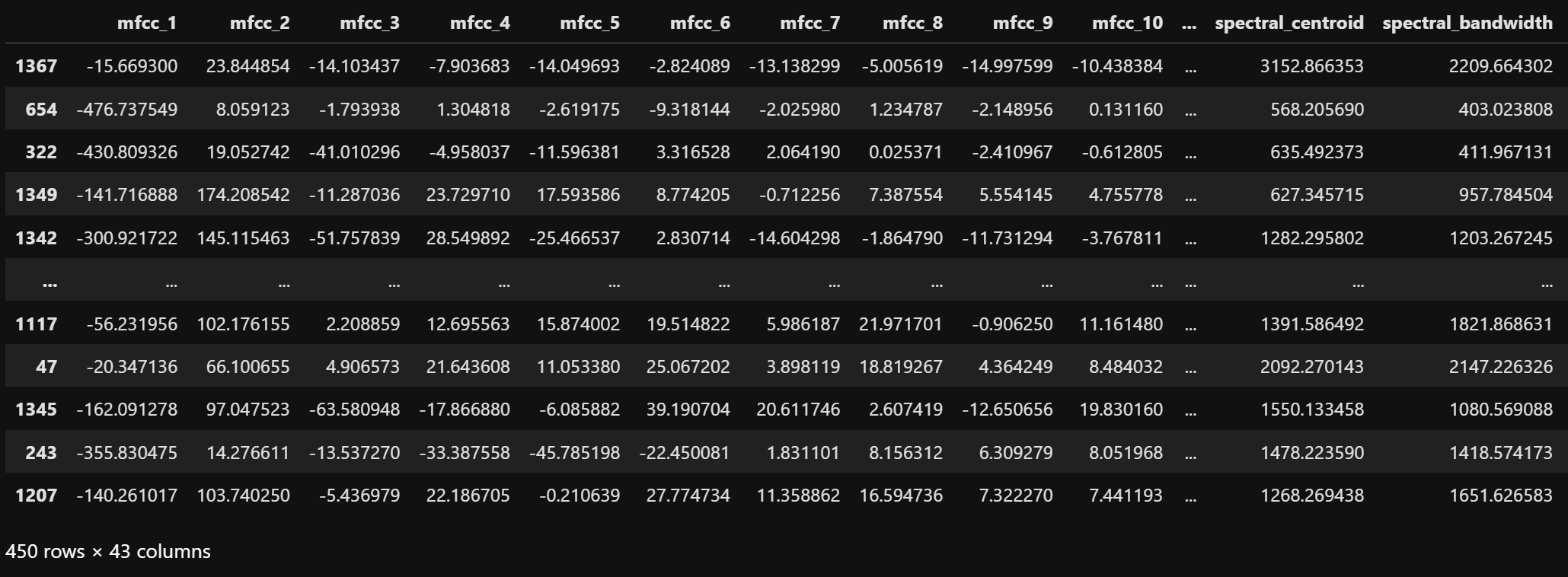
All supervised learning methods require splitting data into training and testing sets to evaluate model performance objectively. This ensures that models are evaluated on data they haven't seen during training, providing a reliable estimate of how well they'll perform on new, unseen data. The dataset is split into training and testing sets in a 7:3 ratio. This means 70% of the dataset is used for training the models, and 30% is used for testing them. The training and testing sets respectively are shown below.
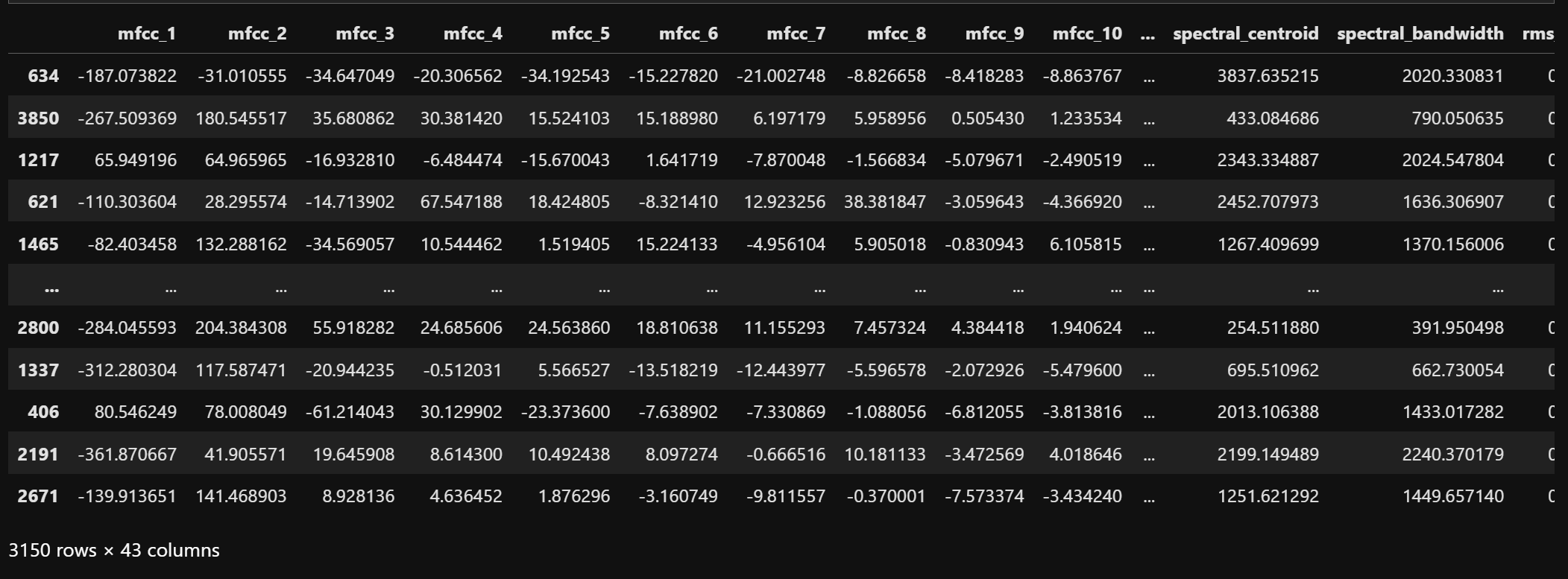
This images depicts the training data, which is split from the original dataset, used for training the model. It contains 70% of the original dataset.
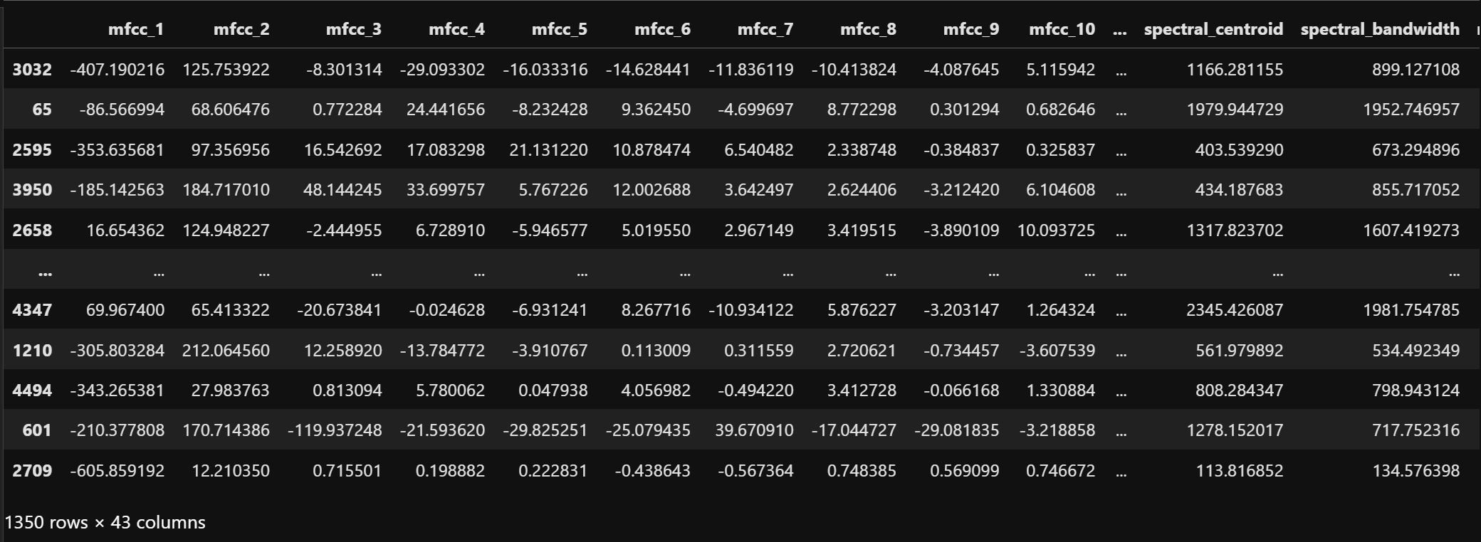
This images depicts the testing data on which the model is tested. It contains 30% of the original dataset.
Three variants of Naive Bayes classifiers are used: MultinomialNB, GaussianNB, and BernoulliNB. Each model has different feature format requirements. The training and testing datasets are transformed according to the models.
Performing Multinomial Naive Bayes Classification
Multinomial Naive Bayes expects discrete feature values. To prepare the data, MinMaxScaler is first applied to scale features between 0 and 1. The scaled values are then multiplied by 100 and rounded to integers. The transformed training and testing sets respectively are shown below.
This images depicts the scaled training data. The features are scaled between 0 and 1 using MinMaxScaler.
This images depicts the scaled testing data. The features are scaled between 0 and 1 using the parameters calculated on the training data.
To make the features discrete numbers, the scaled values are then multiplied by 100 and converted to integers by rounding them off. The discretized training and testing sets respectively are shown below.
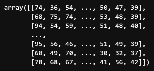
This images depicts the discretized training data. The scaled feature values are now integers between 0 and 100.
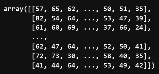
This images depicts the discretized testing data. The scaled feature values are now integers between 0 and 100.
Multinomial Naive Bayes Classification Results
The trained multinomial Naive Bayes model's predictions are tested against the testing data. The performance of the model is evaluated using confusion matrix, classification heatmap, and ROC curve.
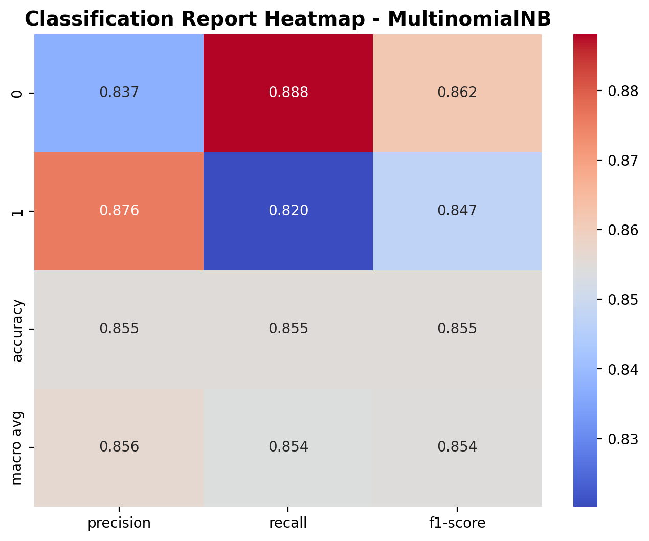
The heatmap shows how well the model performs on both classes: outdoor and music. For class 0 (outdoor), the model achieved a precision of 0.837, recall of 0.888, and F1-score of 0.862. For class 1 (music), the precision was 0.876, recall was 0.820, and F1-score was 0.847. The overall accuracy of the model is 85.5%, and the macro averages for precision, recall, and F1-score are all around 0.85, suggesting that the performance is fairly balanced across both classes.
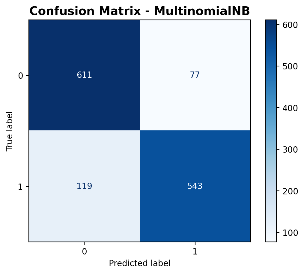
The confusion matrix provides the raw breakdown of predictions. The model correctly predicted 611 outdoor sounds and 543 music sounds. However, it also misclassified 77 outdoor sounds as music and 119 music sounds as outdoor. While the correct predictions outweigh the errors, the misclassification count—especially for music—shows that there’s still room for improvement. The total number of predictions is 1,350, out of which 1,154 were correct.
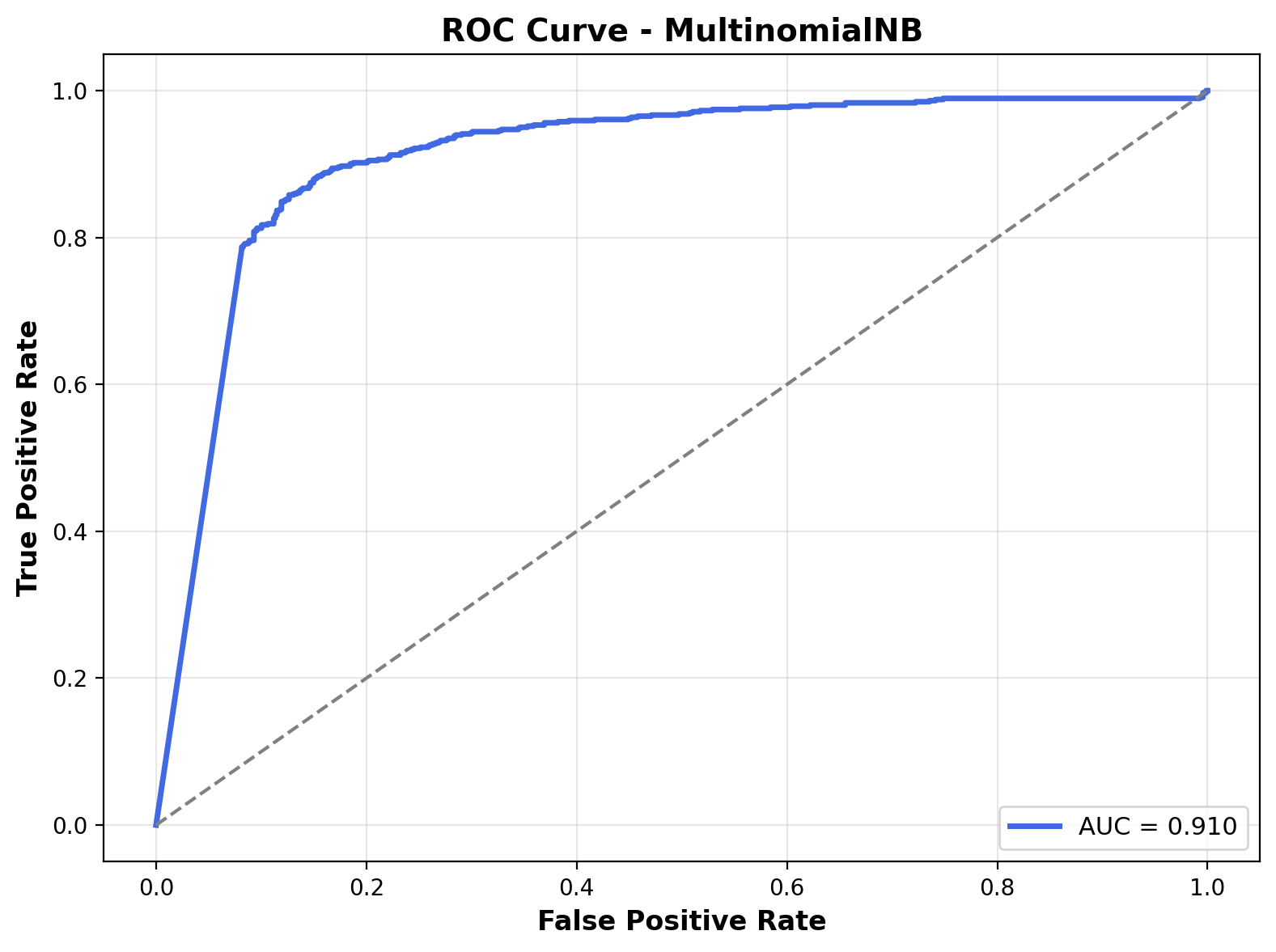
The ROC curve visualizes how well the model can distinguish between the two classes across different thresholds. The curve leans toward the top-left corner, and the Area Under the Curve (AUC) is 0.91, which is quite good. It shows that the model has a strong ability to separate outdoor and music sounds, even if it isn’t perfect. AUC above 0.9 is generally considered very solid for a classifier like this.
Performing Gaussian Naive Bayes Classification
Gaussian Naive Bayes assumes normally distributed features. Therefore, features are standardized using StandardScaler to have zero mean and unit variance. The scaled training and testing datasets respectively are shown below.
This images depicts the scaled training data. The features are scaled to a standard normal distribution with mean=0 and variance=1.
This images depicts the scaled testing data. The features are scaled to a standard normal distribution using parameters calculated on the training data.
Gaussian Naive Bayes Classification Results
The trained Gaussian Naive Bayes model's predictions are tested against the testing data. The performance is evaluated using confusion matrix, classification heatmap, and ROC curve.
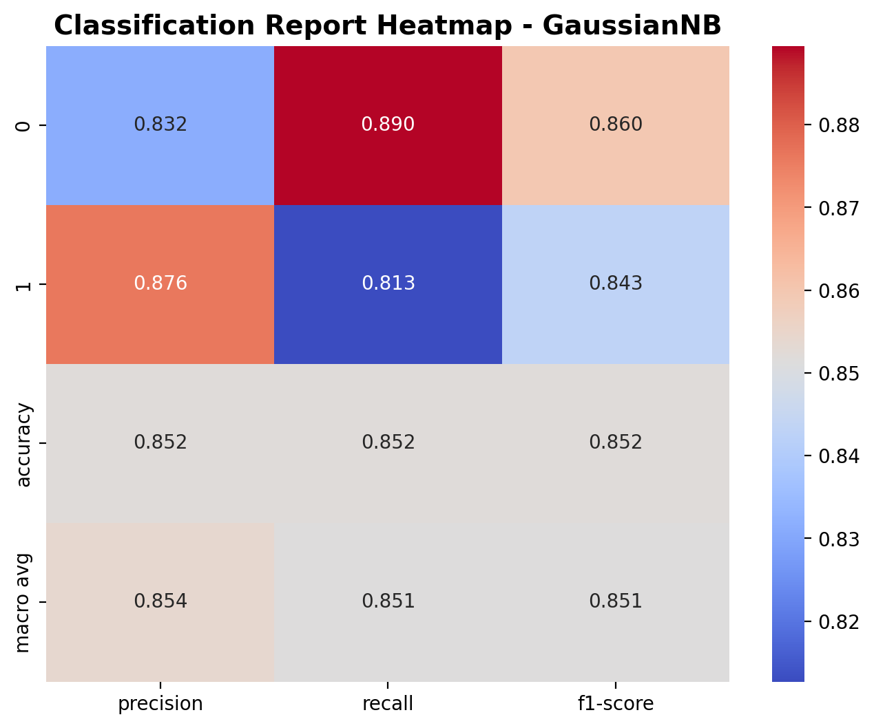
The heatmap highlights the precision, recall, and F1-scores for both outdoor and music classes. For class 0 (outdoor), the precision is 0.832, recall is 0.890, and F1-score is 0.860. For class 1 (music), the precision is 0.876, recall is 0.813, and F1-score is 0.843. These scores indicate the model is relatively balanced in how it handles both classes. The overall accuracy stands at 85.2%, and the macro averages for precision, recall, and F1-score are all close to 0.85, showing consistently decent performance across the board.

The confusion matrix shows that the model correctly predicted 612 outdoor sounds and 538 music sounds. There were 76 outdoor sounds misclassified as music, and 124 music sounds predicted as outdoor. Out of 1,350 total predictions, 1,150 were accurate. The diagonal dominance in the matrix confirms the model is doing a good job, but there’s still a moderate level of confusion between the two classes.

The ROC curve shows the trade-off between true positive rate and false positive rate. The curve for this model rises sharply and stays close to the top-left corner, indicating strong classification ability. The Area Under the Curve (AUC) is 0.922, which means the Gaussian Naive Bayes model is quite effective at separating the two classes overall.
Bernoulli Gaussian Naive Bayes Classification
Bernoulli Naive Bayes requires binary features. Each feature value is binarized: if greater than the mean of that feature, it is set to 1; otherwise, it is set to 0. The binary encoded training and testing datasets respectively are shown below.
This images depicts the binarized training data. The features are encoded to have values of either 1 or 0.
This images depicts the binarized testing data. The features are encoded to have values of either 1 or 0.
Bernoulli Naive Bayes Classification Results
The trained Bernoulli Naive Bayes model's predictions are tested against the testing data. The performance is evaluated using confusion matrix, classification heatmap, and ROC curve.
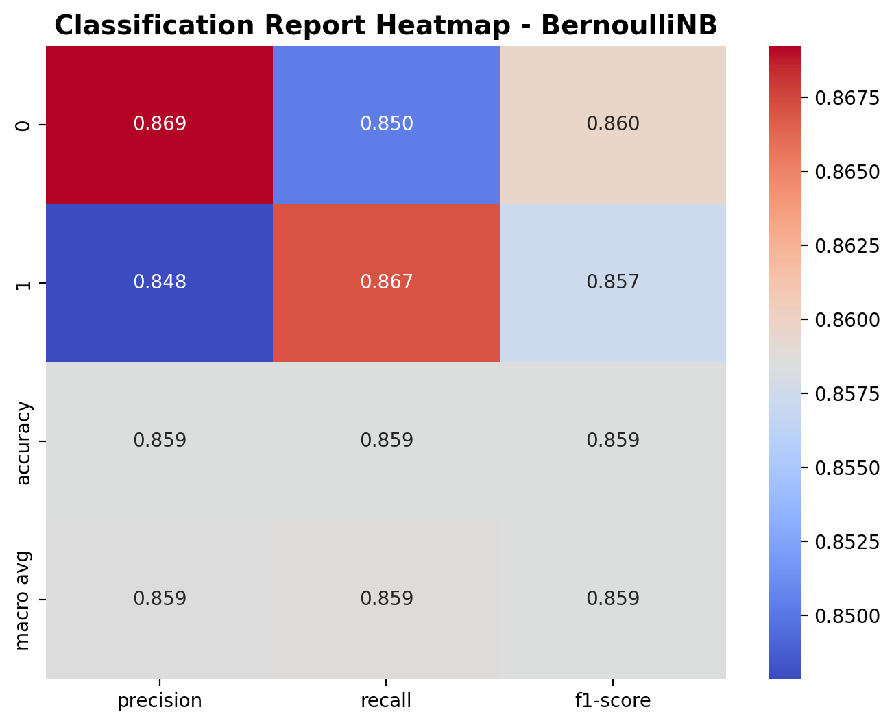
The heatmap shows the model’s classification metrics for both outdoor and music classes. For class 0 (outdoor), the precision is 0.869, recall is 0.850, and F1-score is 0.860. For class 1 (music), the precision is 0.848, recall is 0.867, and F1-score is 0.857. The overall accuracy of the model is 85.9%, and the macro average precision, recall, and F1-scores are all close to 0.86. These values suggest a well-balanced performance, with both classes being handled nearly equally well.
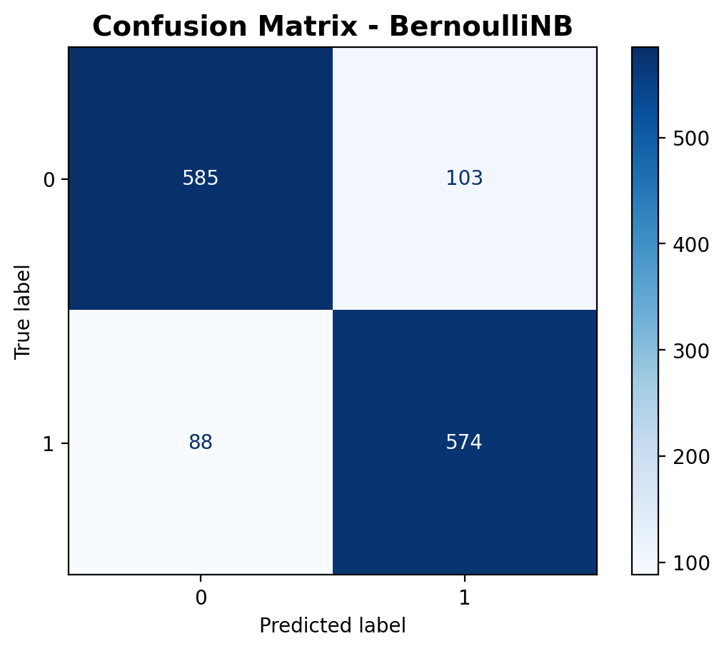
The confusion matrix reveals that the model correctly predicted 585 outdoor sounds and 574 music sounds. It misclassified 103 outdoor samples as music and 88 music samples as outdoor. This totals 1,159 correct predictions out of 1,350. The error rate is fairly low, and the matrix shows the model is reliable for both categories.
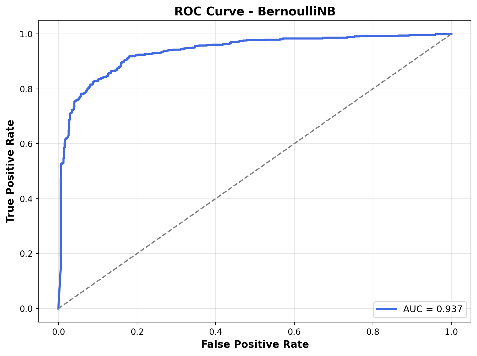
The ROC curve illustrates the model’s ability to distinguish between classes across thresholds. The curve is steep and hugs the top-left corner, indicating excellent separation performance. The Area Under the Curve (AUC) is 0.937, showing that the Bernoulli Naive Bayes model is highly effective at classifying between outdoor and music sounds.
Conclusion
Naive Bayes classifiers performed consistently well in distinguishing between outdoor and music sounds using audio features. All three variants: Multinomial, Gaussian, and Bernoulli, achieved accuracy around 85%, with Bernoulli Naive Bayes performing the best overall. It had the highest F1-score balance between classes and the highest AUC of 0.937, indicating strong classification confidence.
These results suggest that even simple probabilistic models like Naive Bayes can handle audio feature-based classification tasks effectively when features are preprocessed appropriately. The project revealed that audio categories like music and outdoor sounds have distinguishable statistical patterns, which Naive Bayes models are able to capture despite their assumptions of feature independence.
The full script to perform Naive Bayes Classification with its corresponding preprocessing and visualizations can be found here.
Decision Trees
Overview
Decision Trees are versatile supervised learning algorithms that create a model resembling a tree-like structure of decisions. Each internal node represents a "test" on a feature, each branch represents the outcome of the test, and each leaf node represents a class label or a value prediction. Decision Trees are intuitive, easy to interpret, and can handle both classification and regression tasks, making them popular across various domains including finance, healthcare, and computer vision.
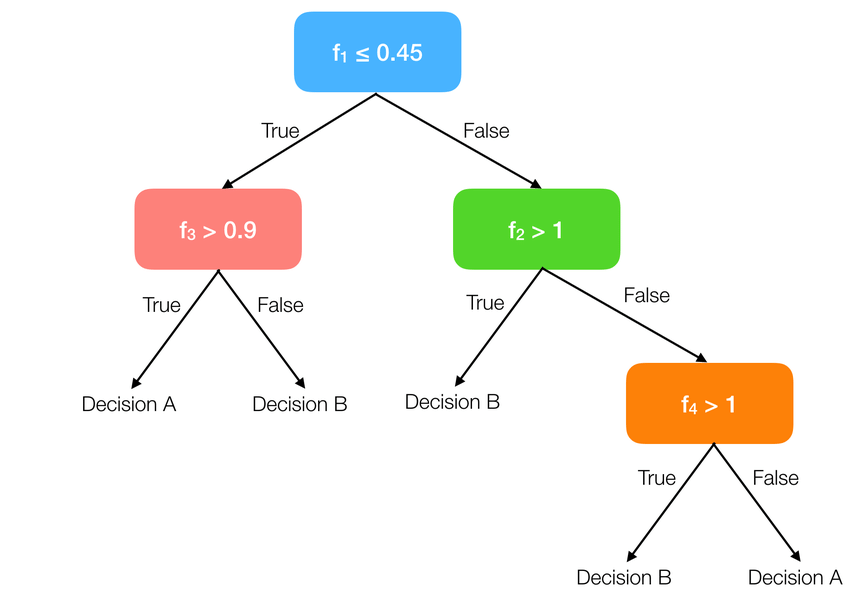
This visualization shows a simple decision tree with 4 features. Starting from the root node (top), the algorithm makes decisions based on features, following different paths until reaching a leaf node that represents a decision category. Each internal node splits the data based on a feature threshold that optimally separates the classes.
Decision Trees work by recursively partitioning the feature space into regions, attempting to find the splits that create the most homogeneous groups with respect to the target variable. To determine the best splits, various impurity measures are used:
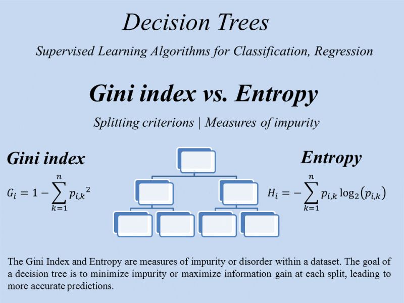
This chart compares Gini Impurity and Entropy, the two most common measures for evaluating splits in classification trees. Both measure class mixing, with lower values indicating better splits. Gini tends to be computationally simpler, while Entropy can sometimes produce more balanced trees. Both reach minimum (0) for pure nodes and maximum for equally mixed nodes.
Impurity Measures and Information Gain
The quality of a split in a Decision Tree is determined by how much it reduces impurity. This reduction is quantified using Information Gain, which measures the difference in entropy (or Gini impurity) before and after a split. Let's understand these concepts with a simple example:
Consider a synthesized dataset with 12 audio samples from three categories: "rain", "fireworks", and "birds". Each sample has a feature "zero_crossing_rate".
- Rain: 4 samples
- Fireworks: 4 samples
- Birds: 4 samples
The decision is to be made regarding whether the data should be split based on the feature "zero_crossing_rate" using a threshold of 0.5.
First, the entropy of the parent node is calculated:
After splitting on "zero_crossing_rate > 0.5", the result is:
- Left child (zero_crossing_rate ≤ 0.5): 6 samples – 4 "rain", 2 "birds"
- Right child (zero_crossing_rate > 0.5): 6 samples – 4 "fireworks", 2 "birds"
Now the entropy of each child node is calculated:
The weighted average entropy after the split is:
Finally, the Information Gain is calculated:
This positive Information Gain of 0.66 indicates that splitting on "zero_crossing_rate > 0.5" is effective in reducing impurity and is a strong candidate for decision making in the tree. The decision tree algorithm would compare this gain with other feature splits and choose the one with the highest gain.
It's worth noting that an infinite number of decision trees can be created for the same dataset by varying:
- The choice of features to split on
- The thresholds for each split
- The order of splits (which feature to use first, second, etc.)
- The depth of the tree
- Pruning strategies to avoid overfitting
This flexibility is both a strength and a challenge, as it allows for highly customized trees but requires careful tuning to avoid overfitting or creating unnecessarily complex models.
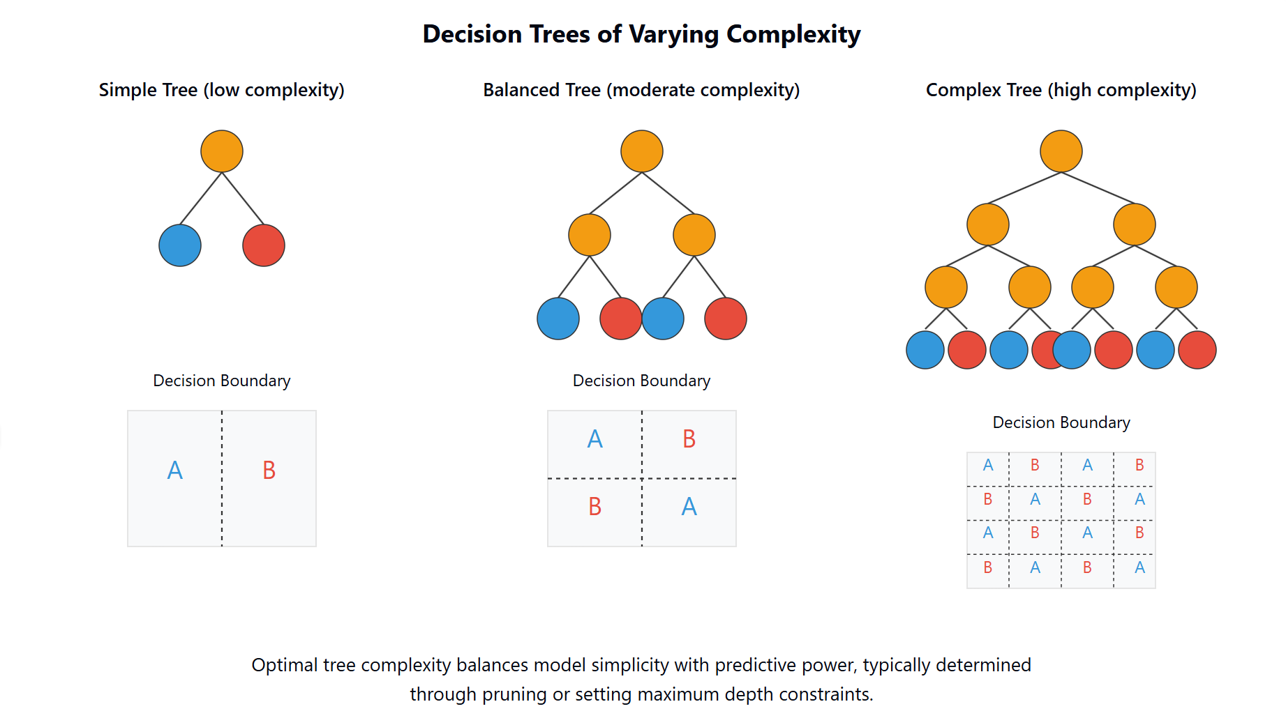
This visualization shows trees of varying complexity: a simple tree with few splits (left), a balanced tree with moderate complexity (middle), and an overfit tree with many splits (right). The optimal tree complexity balances model simplicity with predictive power, typically determined through pruning or setting maximum depth constraints.
Decision Tree Classification of Audio Data
For Decision Tree classification of audio data, audio data from two categories: birds and dog_bark, are used. The dataset is shown below.
The dataset used for Decision Tree analysis includes all 43 acoustic features for the two categories birds and dog_bark.
The label column is encoded into binary form: birds = 1 and dog_bark = 0. This becomes the target variable for the decision tree classification models. The dataset after this transformation is shown below.
The same fundamental approach as with Naive Bayes is used: splitting the dataset into training and testing sets with 70% used for training and 30% used for testing sets using stratified sampling. This train-test split is crucial for objective evaluation of model performance and remains constant across all supervised learning methods for fair comparison. However, Decision Trees have different preprocessing requirements, as they can work with both categorical and numerical features without assumptions about feature distributions. The training and testing sets respectively are shown below.
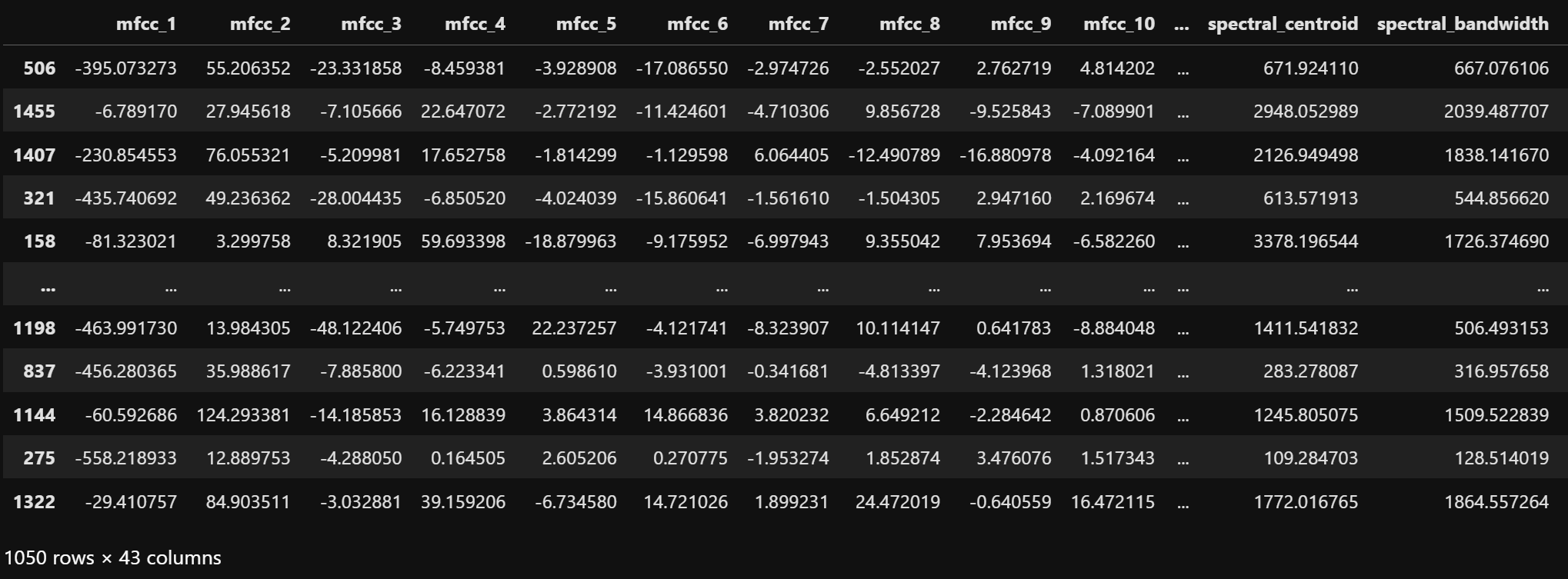
The image shows the training dataset for the decision tree classifiers. It contains 70% of the original dataset.
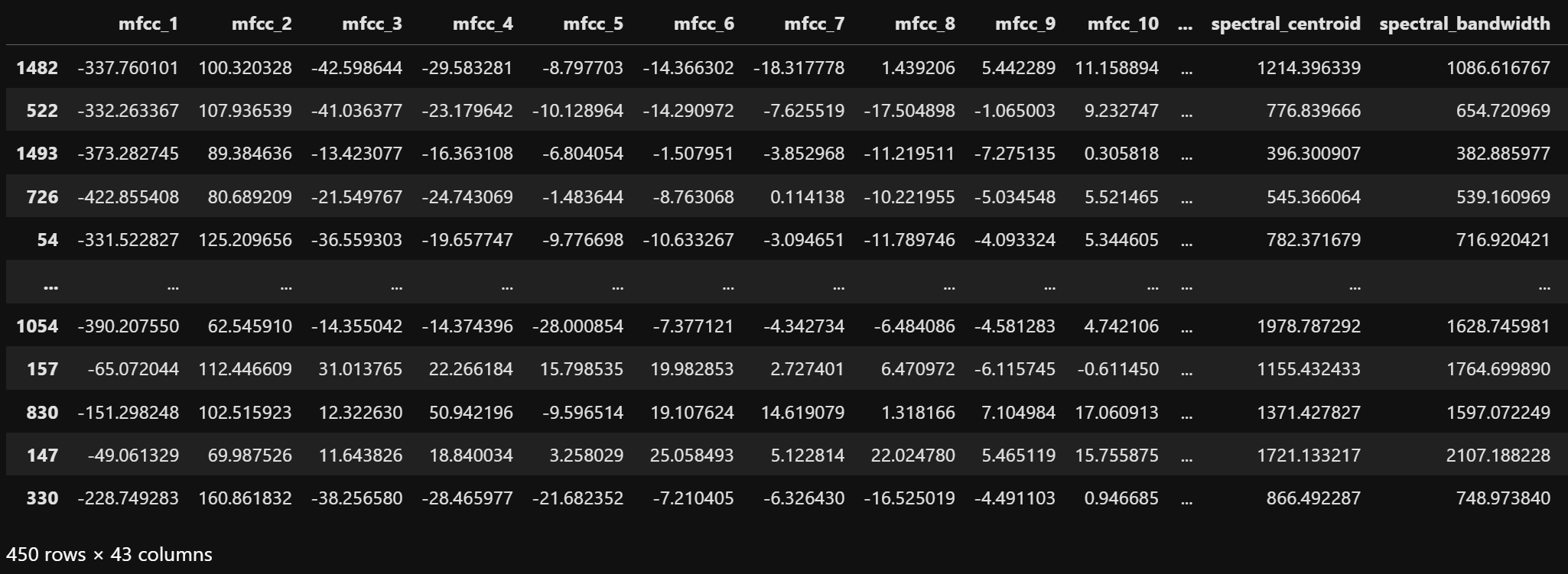
The image shows the testing dataset for the decision tree classifiers. It contains 30% of the original dataset.
Decision Trees can naturally handle continuous features by finding optimal thresholds for splits. The only preprocessing applied was standardization (mean=0, std=1) to ensure features with larger scales don't dominate those with smaller scales during the initial split evaluations. The standardized training and testing datasets respectively are shown below.
The image shows the scaled training dataset for the decision tree classifiers. The features are scaled to a standard normal distribution with mean=0 and variance=1.
The image shows the scaled testing dataset for the decision tree classifiers. The features are scaled to a standard normal distribution using parameters calculated on the training data.
Implementing Decision Trees with Varying Parameters
The implementation of Decision Trees for audio classification uses scikit-learn's DecisionTreeClassifier. Three different trees were created, each with unique hyperparameters to explore how variations in depth, feature selection, and splitting criteria influence the structure and decision paths of the trees:
- Tree 1: Uses the Gini impurity criterion, with a maximum depth of 3 and a maximum of 10 features considered.
- Tree 2: Uses the log loss (cross-entropy) criterion, with a maximum depth of 2 and only 5 features considered.
- Tree 3: Uses the entropy criterion, with a maximum depth of 3 and no restriction on the number of features.
The three Decision Tree models were evaluated on the audio classification task, each revealing different aspects of tree-based learning.
Tree 1 Classification Results
The first tree model's predictions are tested against the testing data. The performance is evaluated using confusion matrix, classification heatmap, and ROC curve.
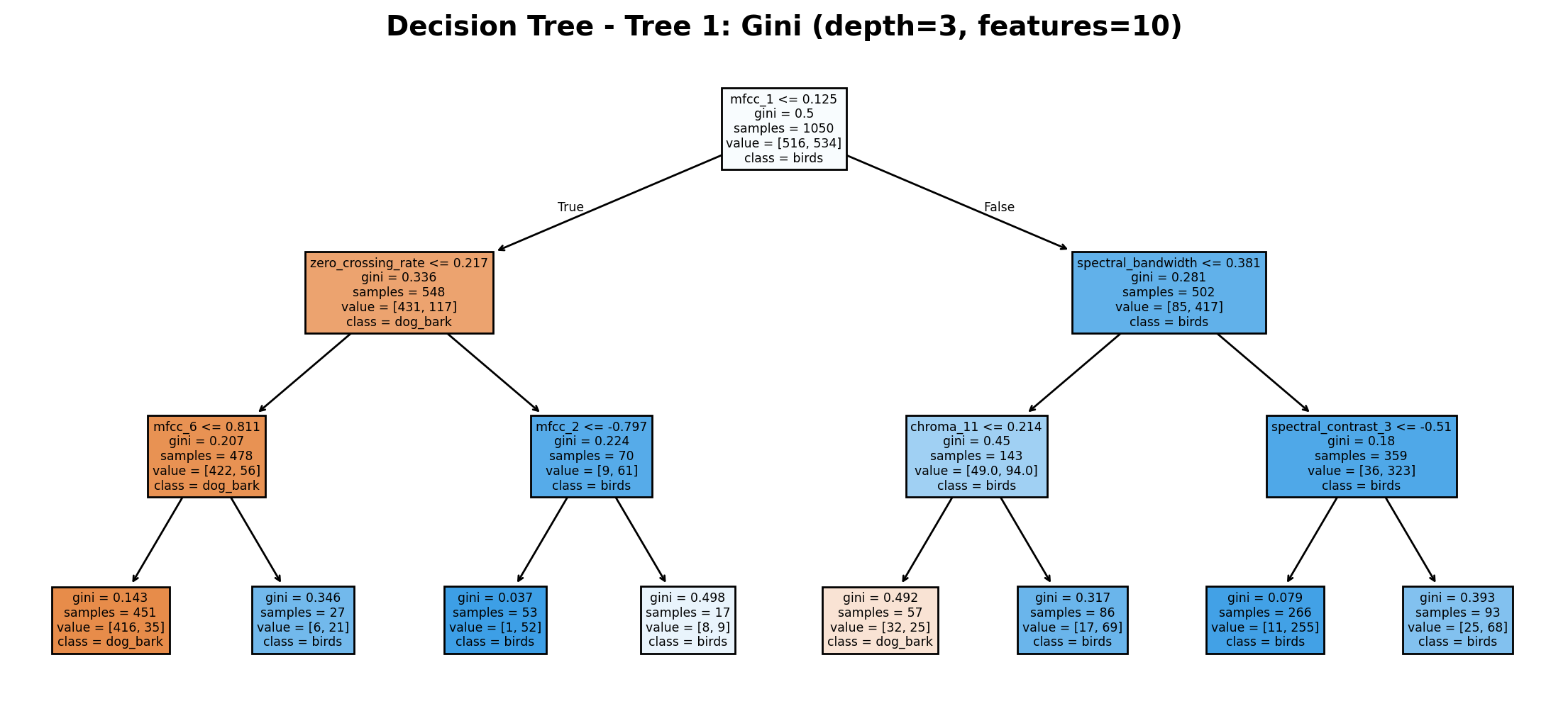
The decision tree uses Gini impurity to classify audio as "birds" or "dog_bark" with a maximum depth of 3 and 10 features. The root node splits on mfcc_1 (threshold 0.125) with 1050 total samples. Key features include zero_crossing_rate (0.217) leading to dog_bark classifications and spectral_bandwidth (0.381) typically leading to birds classifications. Terminal nodes show good separation with low Gini values, demonstrating that acoustic features effectively distinguish between the two sound types.
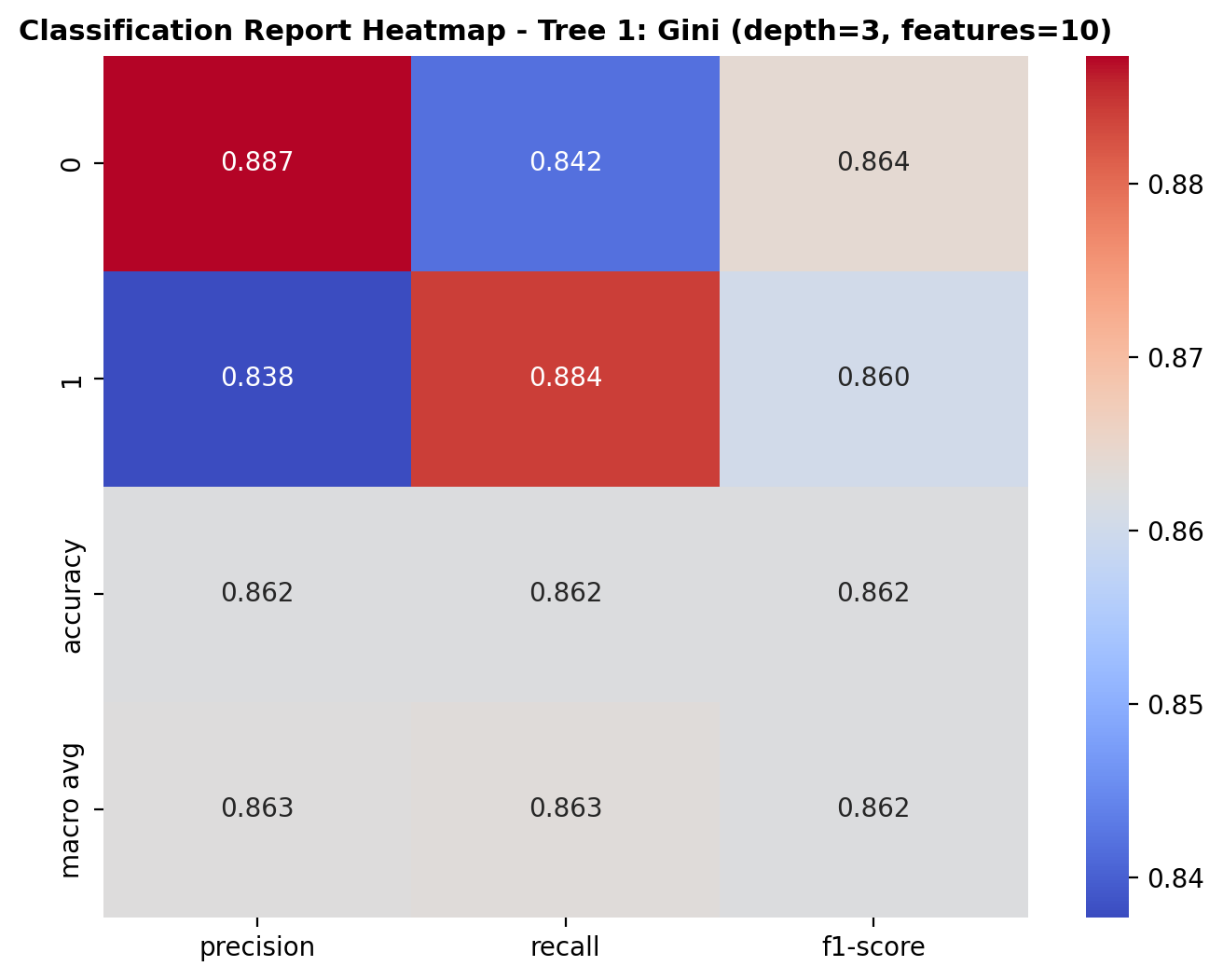
The heatmap summarizes how well the decision tree model performs across the two classes: dog_bark and birds. For class 0 (dog_bark), the precision is 0.887, recall is 0.842, and F1-score is 0.864. For class 1 (birds), the precision is 0.838, recall is 0.884, and F1-score is 0.860. The overall accuracy of the model is 86.2%, and the macro averages for precision, recall, and F1-score are all close to 0.86, indicating balanced classification performance across both classes.
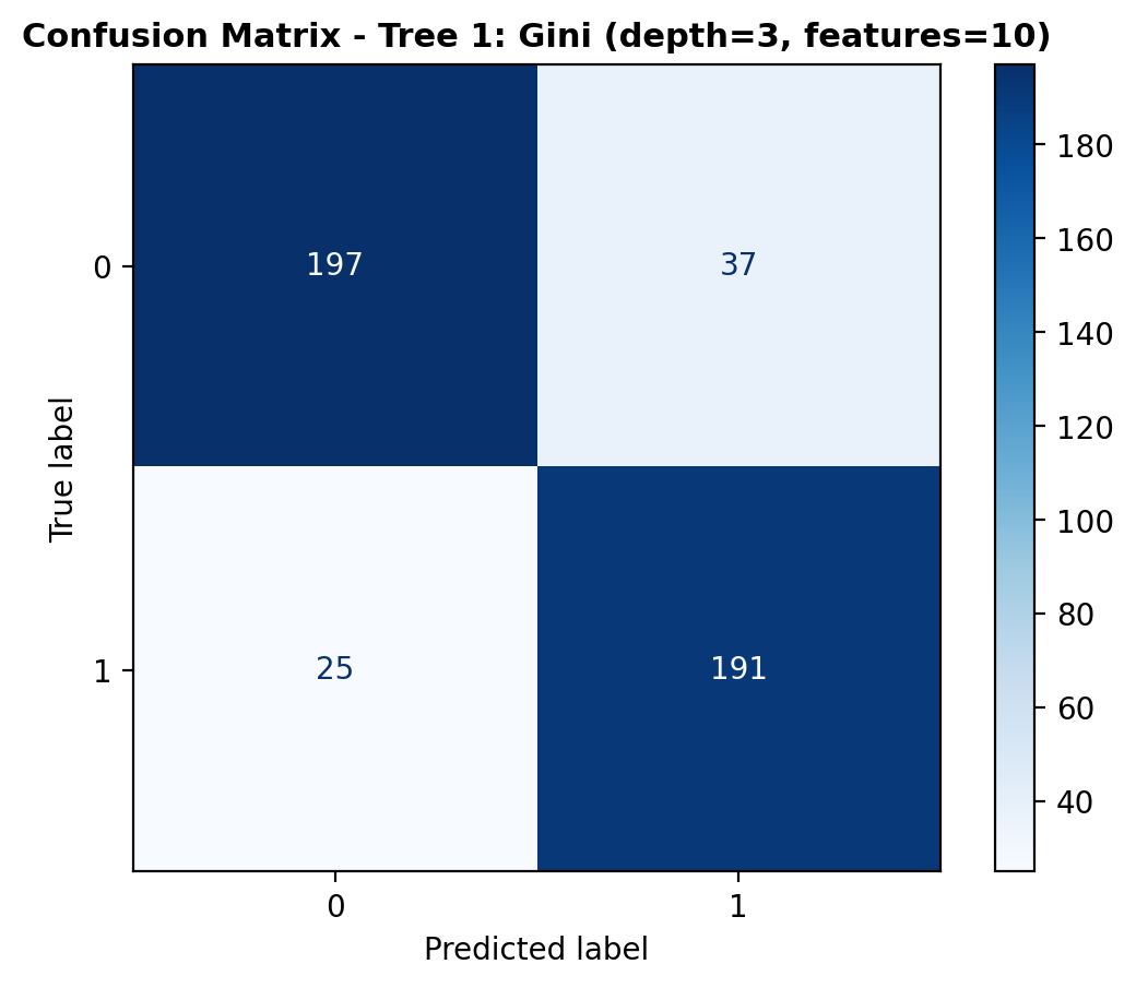
The confusion matrix provides a detailed breakdown of the model’s predictions. The model correctly predicted 197 dog_bark sounds and 191 bird sounds. However, it misclassified 37 dog_bark sounds as birds and 25 bird sounds as dog_bark. While the majority of predictions were accurate, the misclassifications indicate areas where the model could still improve.
The ROC curve shows the model’s ability to distinguish between the two classes across various threshold values. The curve trends toward the top-left corner, and the Area Under the Curve (AUC) is 0.914. This high AUC score reflects the model’s strong capacity to separate dog_bark and bird sounds effectively.
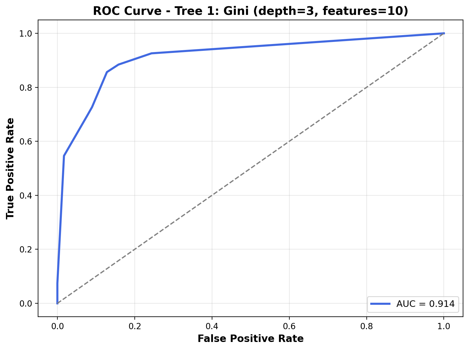
Tree 2 Classification Results
Next, the second tree model's predictions are tested against the testing data. The performance is evaluated using confusion matrix, classification heatmap, and ROC curve.
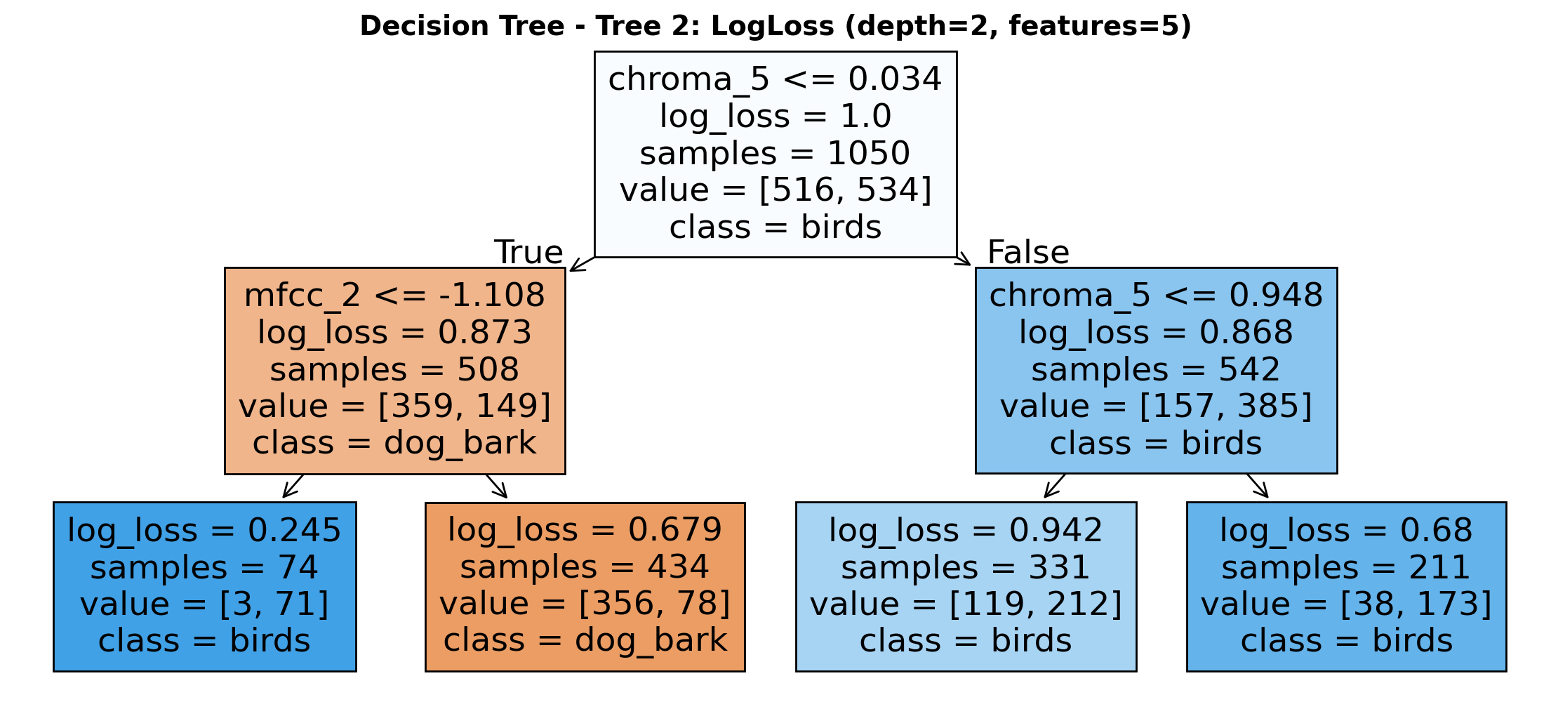
The decision tree uses LogLoss criterion with a maximum depth of 2 and considers only 5 features. The root node splits on chroma_5 (threshold 0.034) with 1050 total samples. When chroma_5 ≤ 0.034, it further splits on mfcc_2 (threshold -1.108) leading primarily to dog_bark classifications. When chroma_5 > 0.034, samples maintain birds classification with most leaf nodes showing decreasing log_loss values. The model efficiently categorizes audio samples using minimal depth while achieving reasonable separation between bird sounds and dog barks.
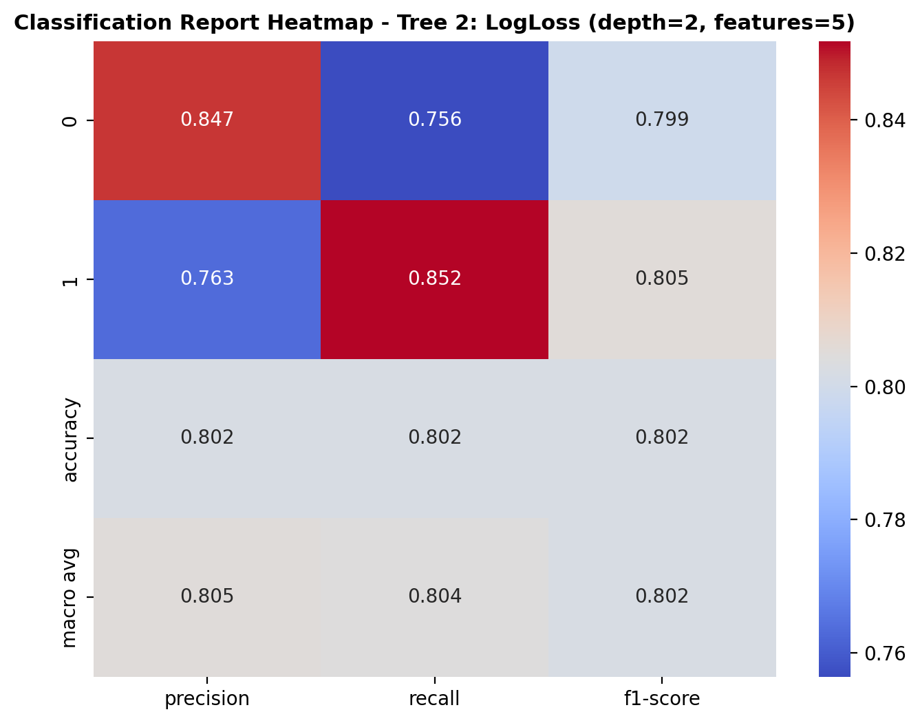
The heatmap shows the performance of the decision tree model (Tree 2) across the two classes: dog_bark and birds. For class 0 (dog_bark), the model achieved a precision of 0.847, recall of 0.756, and F1-score of 0.799. For class 1 (birds), the precision was 0.763, recall was 0.852, and F1-score was 0.805. The overall accuracy of the model is 80.2%, and the macro-averaged precision, recall, and F1-score are all close to 0.80, indicating balanced but slightly reduced performance compared to deeper trees.
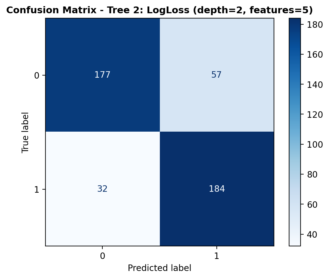
The confusion matrix shows how the model’s predictions are distributed. The model correctly identified 177 dog_bark sounds and 184 bird sounds. However, 57 dog_bark samples were misclassified as birds, while 32 bird sounds were labeled as dog_bark. While the model shows reasonable accuracy, the higher misclassification of dog_bark samples suggests room for improvement.
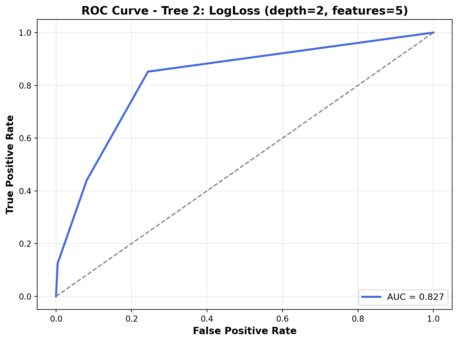
The ROC curve illustrates the trade-off between the true positive rate and false positive rate at various thresholds. For this model, the curve has a noticeable upward bend but doesn’t sharply hug the top-left corner, and the Area Under the Curve (AUC) is 0.827. This AUC value suggests that while the model can distinguish between classes reasonably well, its discriminative ability is slightly lower than Tree 1.
Tree 3 Classification Results
Finally, the third tree model's predictions are tested against the testing data. The performance is evaluated using confusion matrix, classification heatmap, and ROC curve.
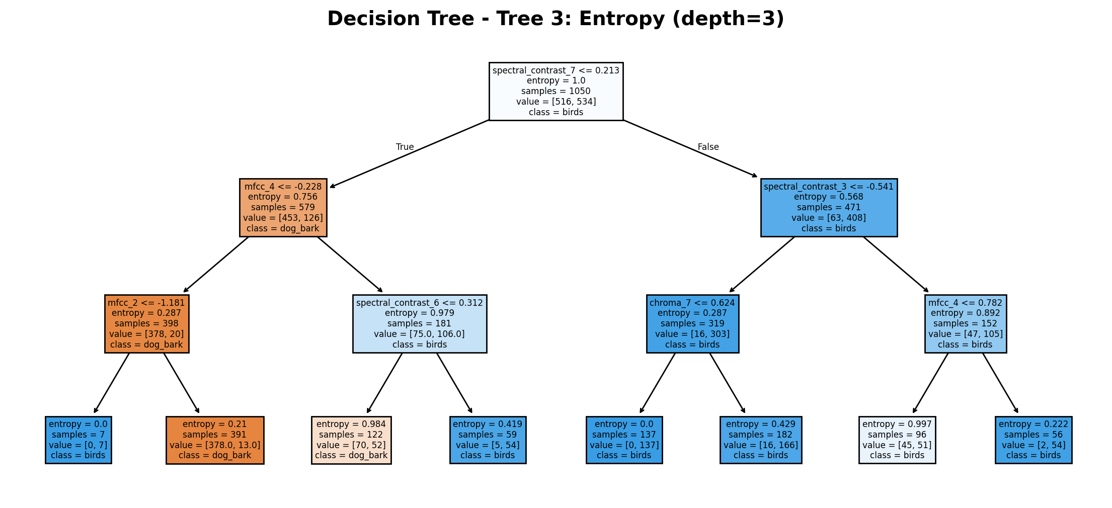
The decision tree uses Entropy criterion with a maximum depth of 3 and no feature restrictions. The root node splits on spectral_contrast_7 (threshold 0.213) with 1050 total samples. Key features include mfcc_4 (threshold -0.228) leading to dog_bark classifications and spectral_contrast_3 (threshold -0.541) typically resulting in birds classifications. Several terminal nodes achieve perfect separation (entropy = 0.0), particularly in the bird classification branches. The tree effectively leverages acoustic spectral features and MFCCs to distinguish between the two sound types.
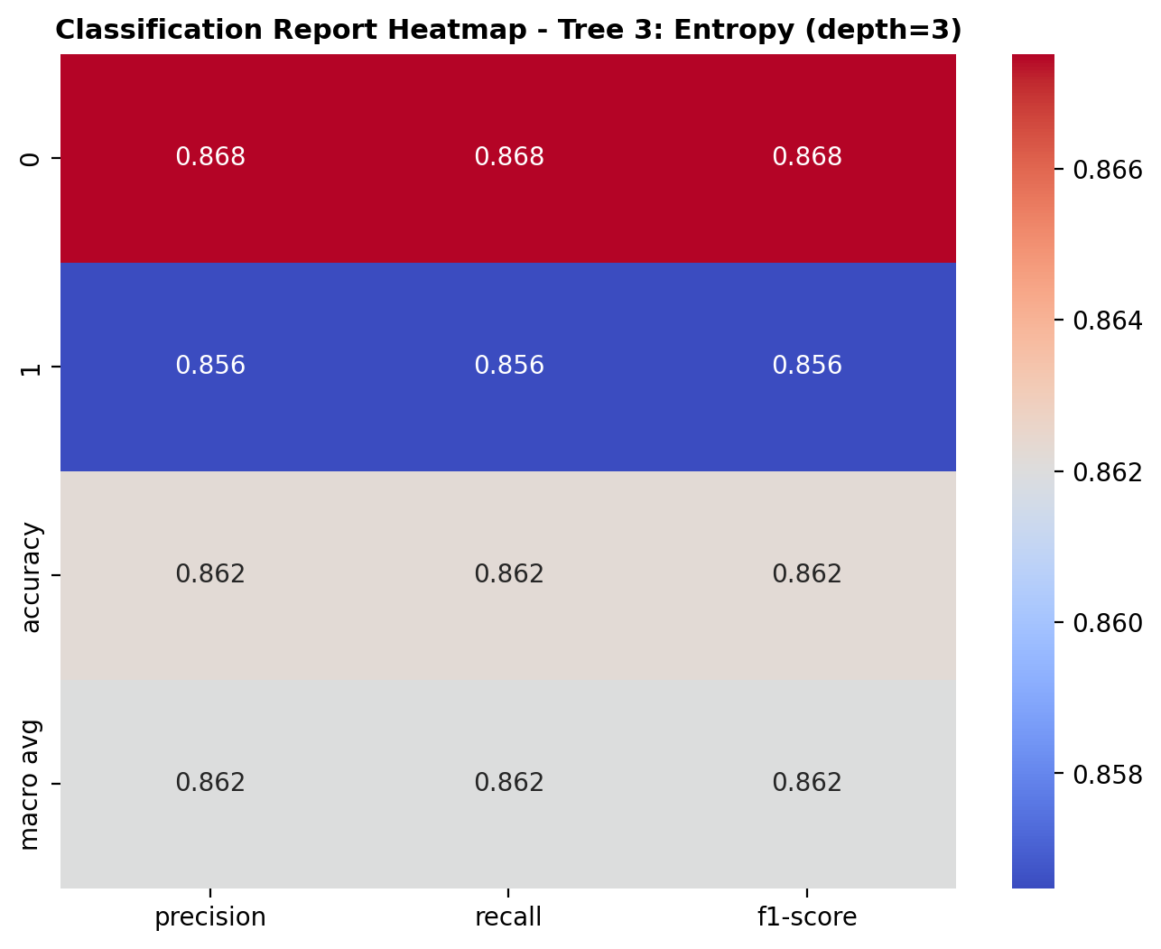
The heatmap summarizes the classification performance of the decision tree model (Tree 3) across dog_bark and bird sounds. For class 0 (dog_bark), the model achieved a precision of 0.868, recall of 0.868, and F1-score of 0.868. For class 1 (birds), the precision was 0.856, recall was 0.856, and F1-score was 0.856. The overall accuracy of the model is 86.2%, and the macro averages for precision, recall, and F1-score are all 0.862, indicating consistent and balanced performance between the two classes.
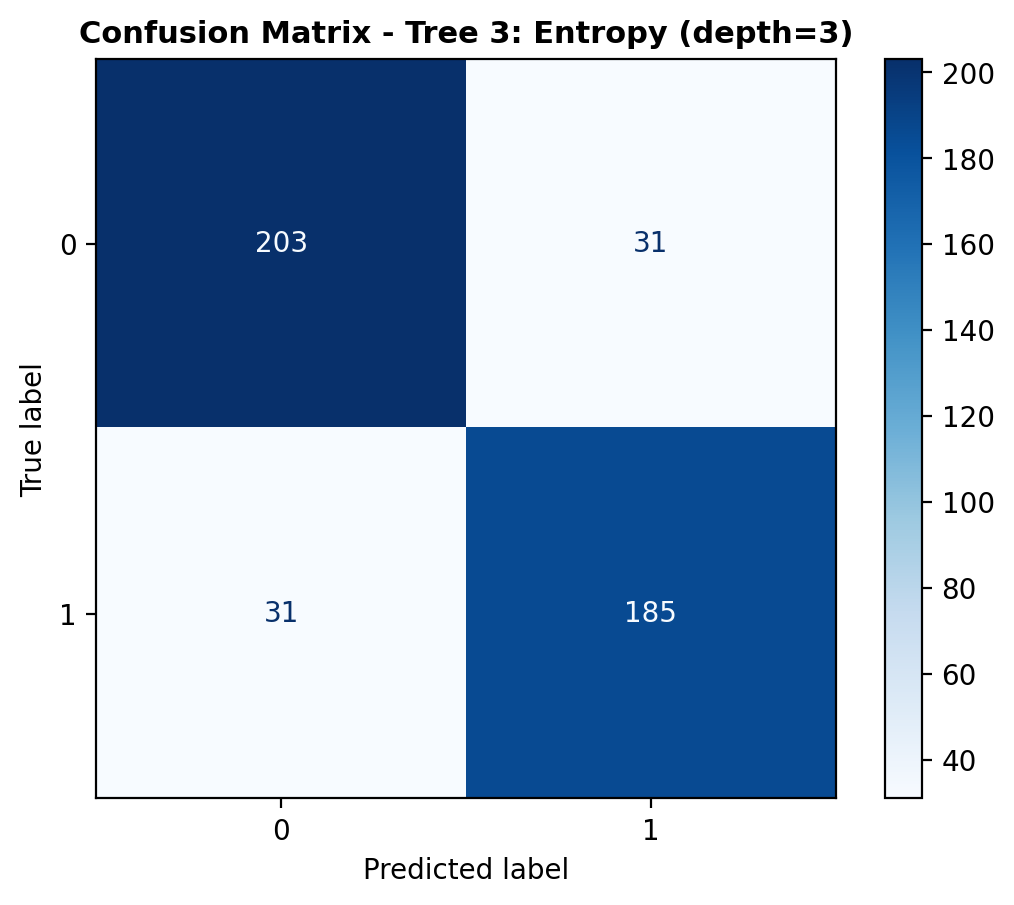
The confusion matrix shows that the model correctly classified 203 dog_bark sounds and 185 bird sounds. However, it also misclassified 31 samples from each class, with dog_bark sounds predicted as birds and vice versa. Despite these misclassifications, the model made 388 correct predictions out of 450 total, reflecting strong reliability in identifying both categories.
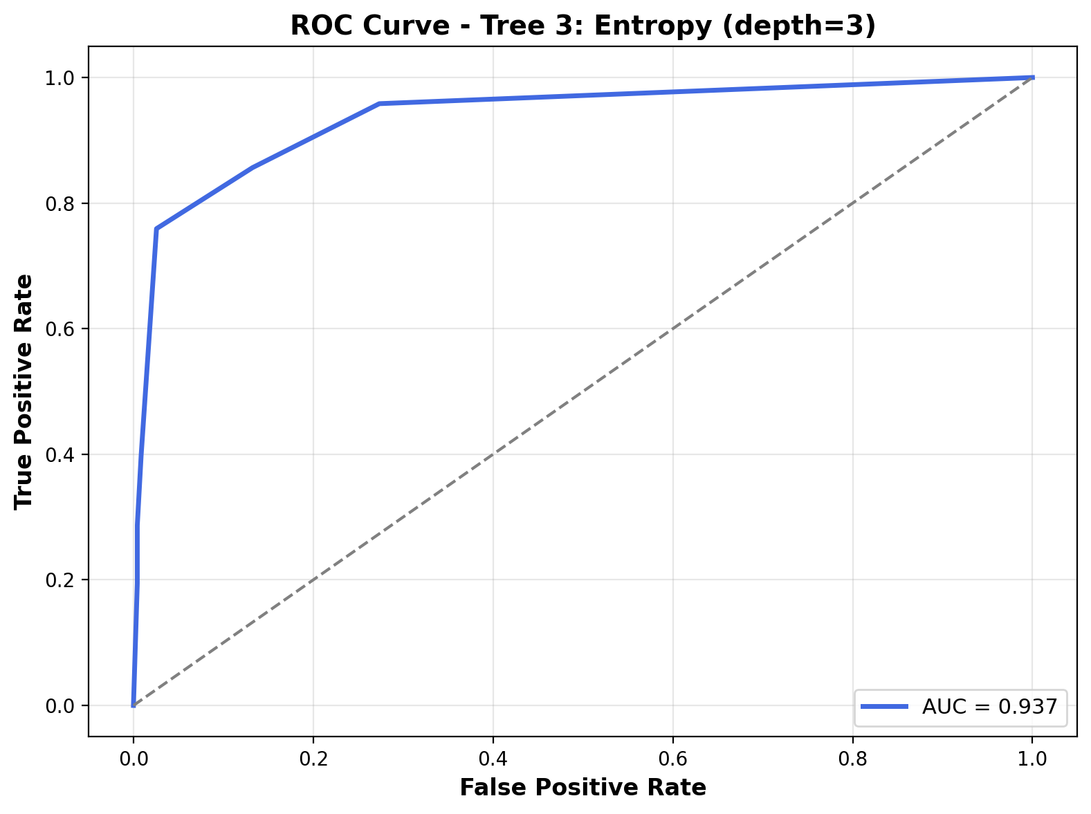
The ROC curve highlights the model’s strong ability to differentiate between the two classes. The curve hugs the top-left corner closely, and the Area Under the Curve (AUC) is 0.937, the highest among the three trees. This indicates excellent discriminative performance, with the model maintaining high sensitivity and specificity across thresholds.
Conclusion
Decision Tree classifiers demonstrated solid performance in classifying between bird and dog_bark sounds based on extracted audio features. All three trees—using Gini, LogLoss, and Entropy as splitting criteria—achieved accuracy between 80% and 86%, with Tree 3 (Entropy, depth=3) performing the best overall. It had the most balanced precision and recall across classes and the highest AUC of 0.937, indicating excellent class separation capability.
These results highlight the interpretability and flexibility of decision trees, especially when working with structured feature sets. Even shallow trees with limited depth were able to capture meaningful distinctions between sound types, showing that hierarchical rule-based models can be effective for sound classification when the features are informative.
The full script to run Decision Tree Classification along with preprocessing and evaluation visualizations is available here.
Regression
Linear Regression
Linear regression is a supervised learning algorithm that models the relationship between a dependent variable and one or more independent variables by fitting a linear equation to the observed data. The model assumes a linear relationship where the output is a weighted sum of the input features plus a bias term. Linear regression is primarily used for predicting continuous values and estimating the strength of relationships between variables. Its simplicity, interpretability, and computational efficiency make it a foundational technique in statistics and machine learning.
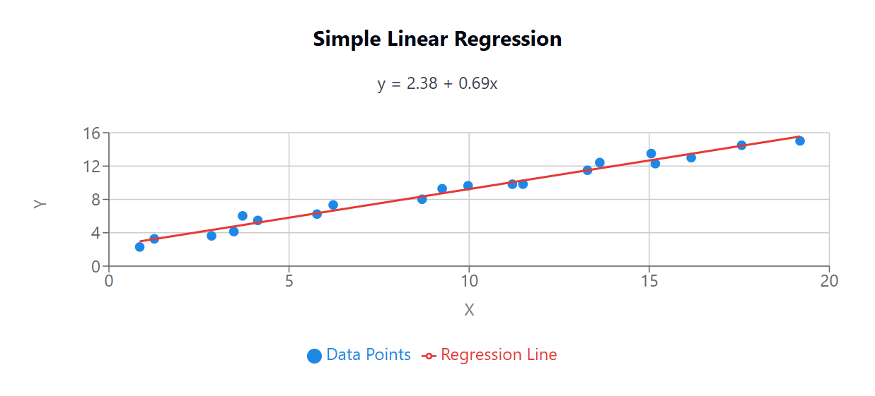
This visualization shows a simple linear regression with one input feature. The blue points represent data samples, and the red line represents the linear model that minimizes the sum of squared differences between predicted and actual values. The equation of the line is typically expressed as y = β₀ + β₁x, where β₀ is the intercept and β₁ is the slope.
Logistic Regression
Logistic regression is a supervised learning algorithm used for binary classification problems. Despite its name, it's a classification algorithm rather than a regression technique. Logistic regression models the probability that an instance belongs to a particular class using the logistic function (sigmoid) to transform a linear combination of features into a value between 0 and 1. This probability can then be thresholded to make binary predictions. Logistic regression is widely used in fields like medicine, marketing, and risk assessment for its interpretable results and probability estimates.
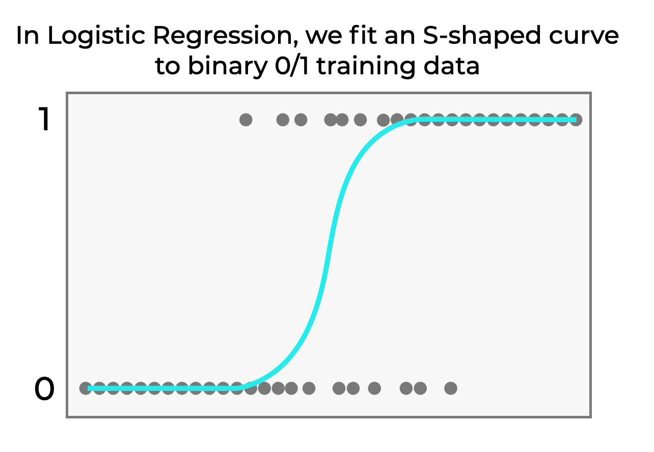
This visualization illustrates logistic regression for binary classification. The gray dots represent binary training data points (0 or 1), and the cyan S-shaped curve shows how logistic regression fits a sigmoid function to this data. The curve models the probability of the positive class (1) based on the input feature, transitioning smoothly from 0 to 1.
Similarities and Differences
While linear and logistic regression differ in output type and application, they share several foundational traits:
- Both are supervised learning algorithms used for predictive modeling.
- They rely on a linear combination of input features.
- They can be regularized using techniques like L1 (Lasso) or L2 (Ridge).
- Both models are computationally efficient and offer interpretable coefficients.
- They use gradient-based optimization when closed-form solutions are impractical.
However, both of these serve fundamentally different purposes:
| Aspect | Linear Regression | Logistic Regression |
|---|---|---|
| Purpose | Predicts continuous numerical values | Predicts probabilities for classification |
| Output Range | Unbounded (any real number) | Bounded between 0 and 1 |
| Transformation Function | None (linear combination of inputs) | Sigmoid function |
| Loss Function | Mean Squared Error | Cross-Entropy Loss |
| Optimization Method | Closed-form solution or gradient descent | Typically gradient descent |
| Interpretability | Coefficients represent change in output per unit change in input | Coefficients represent log-odds ratios |
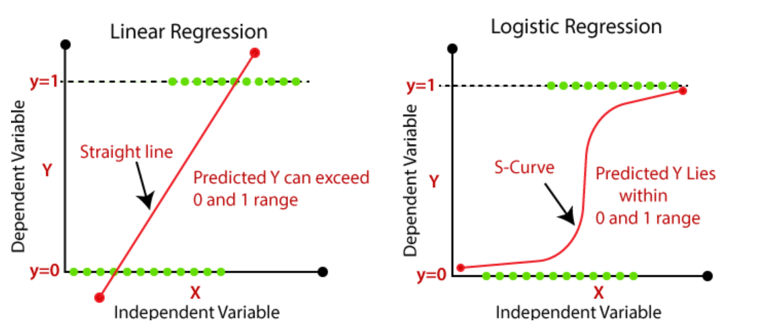
This visualization compares linear and logistic regression models. The straight line represents linear regression, extending beyond the [0, 1] range and predicting continuous values. In contrast, the S-shaped curve represents logistic regression, which maps inputs to probabilities using a sigmoid function. While linear regression is suited for predicting numeric outputs, logistic regression is ideal for binary classification tasks where outputs represent probabilities between 0 and 1.
The Sigmoid Function in Logistic Regression
Logistic regression uses the sigmoid function as its key component. The sigmoid function transforms the linear combination of input features into a probability value between 0 and 1. It has an S-shaped curve defined by the equation: $$\sigma(z) = \frac{1}{1 + e^{-z}}$$ where \( z \) is the linear combination of features. The sigmoid function solves a fundamental problem: while linear regression outputs can range from negative infinity to positive infinity, probabilities must be bounded between 0 and 1. The function's shape also creates a natural decision boundary at 0.5 probability.
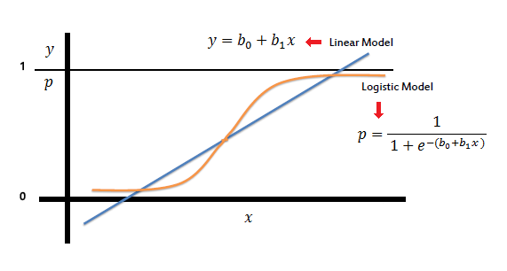
This graph shows how the sigmoid function transforms a linear model into a logistic model. The sigmoid function $$p = \frac{1}{1 + e^{-(b₀+b₁x)}}$$ maps the linear predictor (blue line) to probability values between 0 and 1 (orange curve).
Maximum Likelihood and Logistic Regression
Maximum likelihood estimation (MLE) is the statistical principle underlying logistic regression training. While linear regression minimizes the sum of squared errors, logistic regression maximizes the likelihood of observing the given data under the model's probability distributions. The likelihood function measures how probable the observed data is given the current model parameters. For each data point, logistic regression computes the probability of the observed class, and the goal is to find parameter values that maximize the product of these probabilities (or, equivalently, the sum of log probabilities). This approach naturally leads to the cross-entropy loss function used in logistic regression and provides not just class predictions but well-calibrated probability estimates.
Logistic Regression for Audio Data
For Logistic Regression classification of audio data, sound samples from two categories sirens and fireworks, are selected to construct a binary classification problem. These categories offer clear contrast in acoustic profiles, making them suitable for this task. The dataset is shown below.
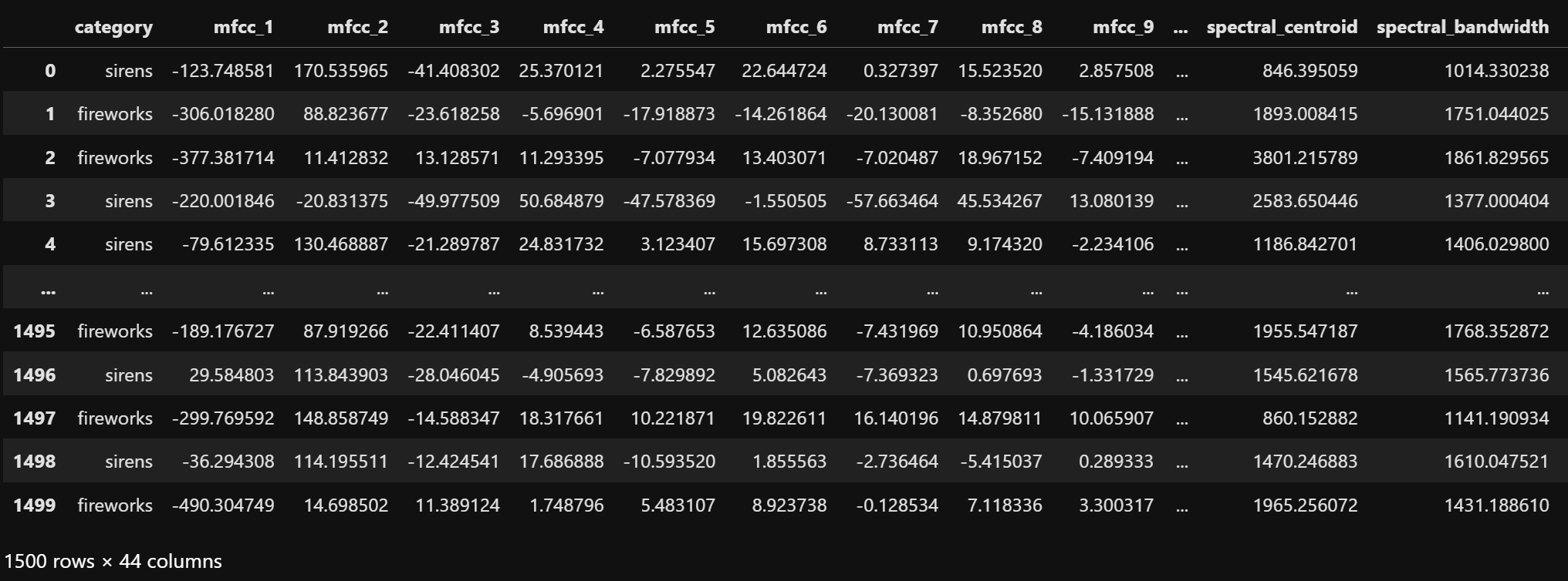
The dataset includes 43 extracted acoustic features for both sirens and fireworks. Each row represents one sound instance, with numerical values corresponding to different audio descriptors.
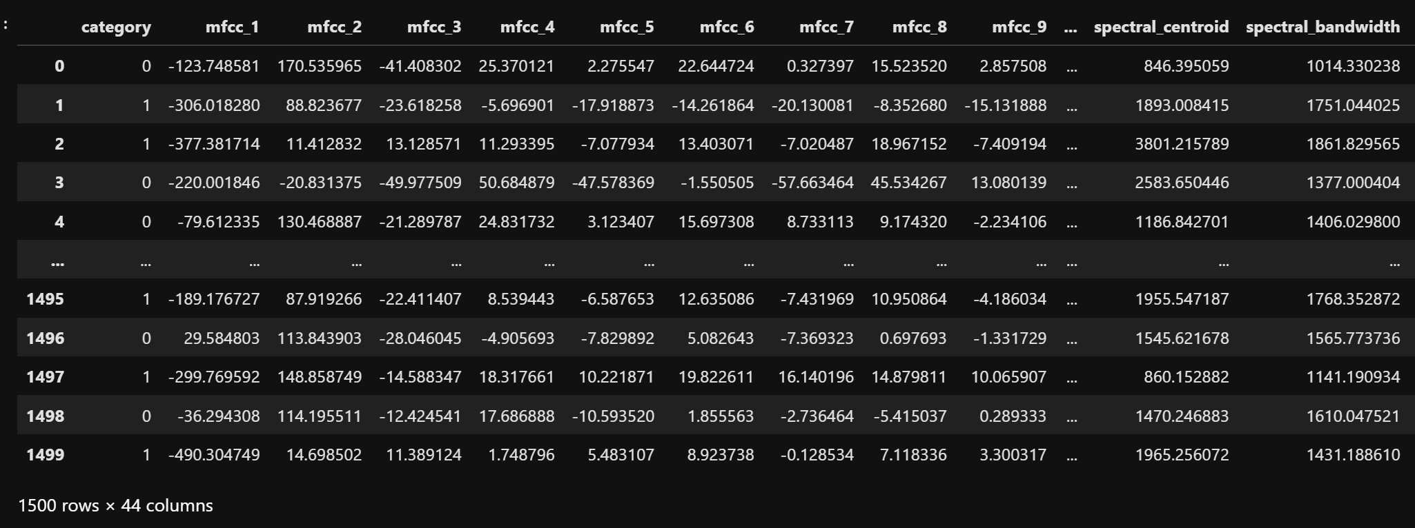
The label column is converted into binary format: sirens = 0 and fireworks = 1. This binary label becomes the target variable for model training. The dataset after this transformation is shown below.
The dataset is split using stratified sampling to ensure class balance: 70% is used for training and 30% for testing. This same split is maintained across all supervised classification models for consistency. The split training and testing datasets respectively are shown below.
The training dataset contains 70% of the original samples. It is used to fit the model.
The testing dataset comprises the remaining 30% and is used to evaluate model generalization performance.
To evaluate how well Logistic Regression performs compared to a probabilistic baseline, it is benchmarked against a Multinomial Naive Bayes model.
Since Multinomial Naive Bayes expects discrete inputs, a shared preprocessing pipeline is applied: feature values are scaled to the [0, 1] range using MinMaxScaler, multiplied by 100, and converted to integers.
This transformation allows both models to operate on the same discretized representation for a fair comparison. The scaled and discretized training and testing sets are shown below.
The training dataset after discretization. All features are scaled to [0, 1], multiplied by 100, and converted to integers for compatibility with Multinomial Naive Bayes.
The testing dataset undergoes the same transformation using parameters learned from the training data.
Logistic Regression Classification Results
The performance of the Logistic Regression model is evaluated on the binary classification task involving sirens and fireworks. The evaluation uses a confusion matrix, a classification heatmap, and a ROC curve to assess model effectiveness.
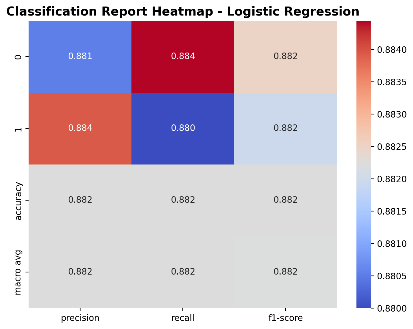
The heatmap shows the classification report for the logistic regression model. For class 0 (sirens), the precision is 0.881, recall is 0.884, and F1-score is 0.882. For class 1 (fireworks), the precision is 0.884, recall is 0.880, and F1-score is 0.882. The overall accuracy is 88.2%, with macro-averaged precision, recall, and F1-score all equal to 0.882, indicating strong and balanced performance across both classes.
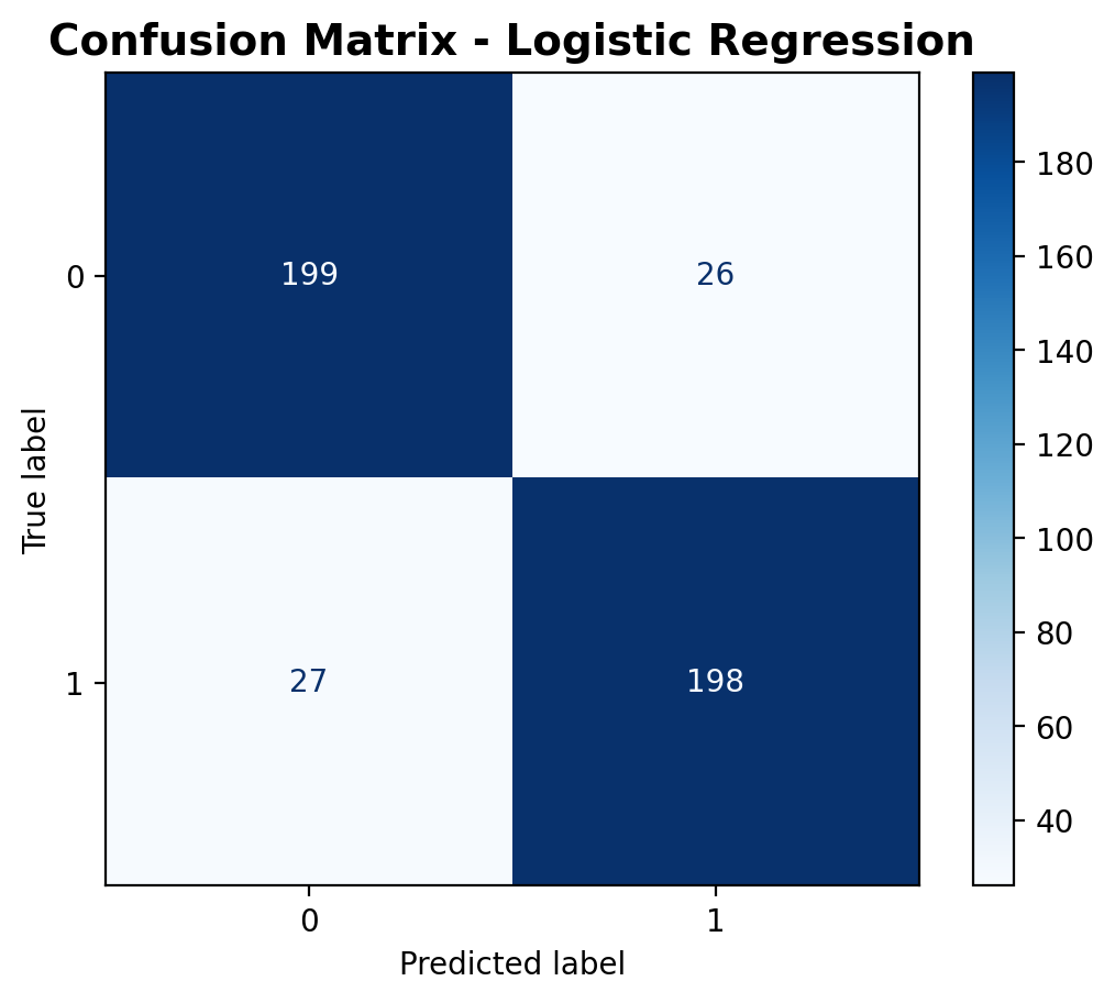
The confusion matrix summarizes the model’s prediction distribution. The model correctly identified 199 siren samples and 198 fireworks samples. It misclassified 26 fireworks as sirens and 27 sirens as fireworks. The distribution of errors is fairly symmetrical, indicating balanced misclassification.
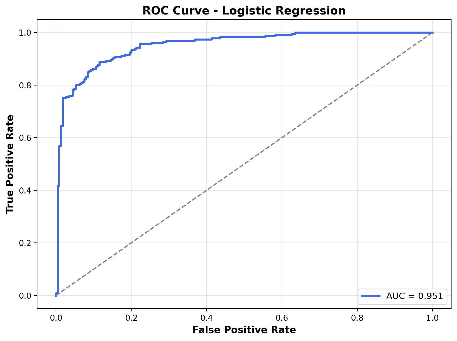
The ROC curve illustrates the trade-off between the true positive rate and false positive rate across different thresholds. The curve closely hugs the top-left corner, demonstrating strong class separability. The Area Under the Curve (AUC) is 0.951, indicating excellent discriminative capability of the logistic regression model.
Comparitive Multinomial Naive Bayes Classification Results
The Multinomial Naive Bayes model is also trained on the same binary classification task. This model is also evaluated using standard performance metrics including a confusion matrix, classification report heatmap, and ROC curve.
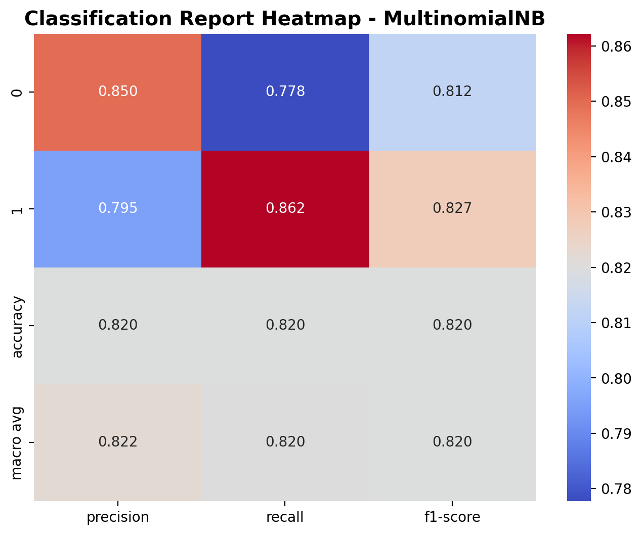
The classification report highlights the performance of the Multinomial Naive Bayes model. For class 0 (sirens), the precision is 0.850, recall is 0.778, and F1-score is 0.812. For class 1 (fireworks), the precision is 0.795, recall is 0.862, and F1-score is 0.827. The overall accuracy is 82.0%, with macro average precision, recall, and F1-score around 0.82. While the model performs reasonably well, these scores are slightly lower than those achieved by the logistic regression model, which had a higher accuracy and more balanced precision-recall performance.
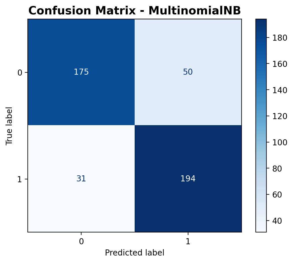
The confusion matrix shows that the model correctly classified 175 siren samples and 194 fireworks samples. However, it misclassified 50 fireworks as sirens and 31 sirens as fireworks. Compared to the logistic regression model—which had fewer false positives and false negatives—the Multinomial Naive Bayes model makes more errors, particularly in predicting the siren class, leading to a drop in precision.
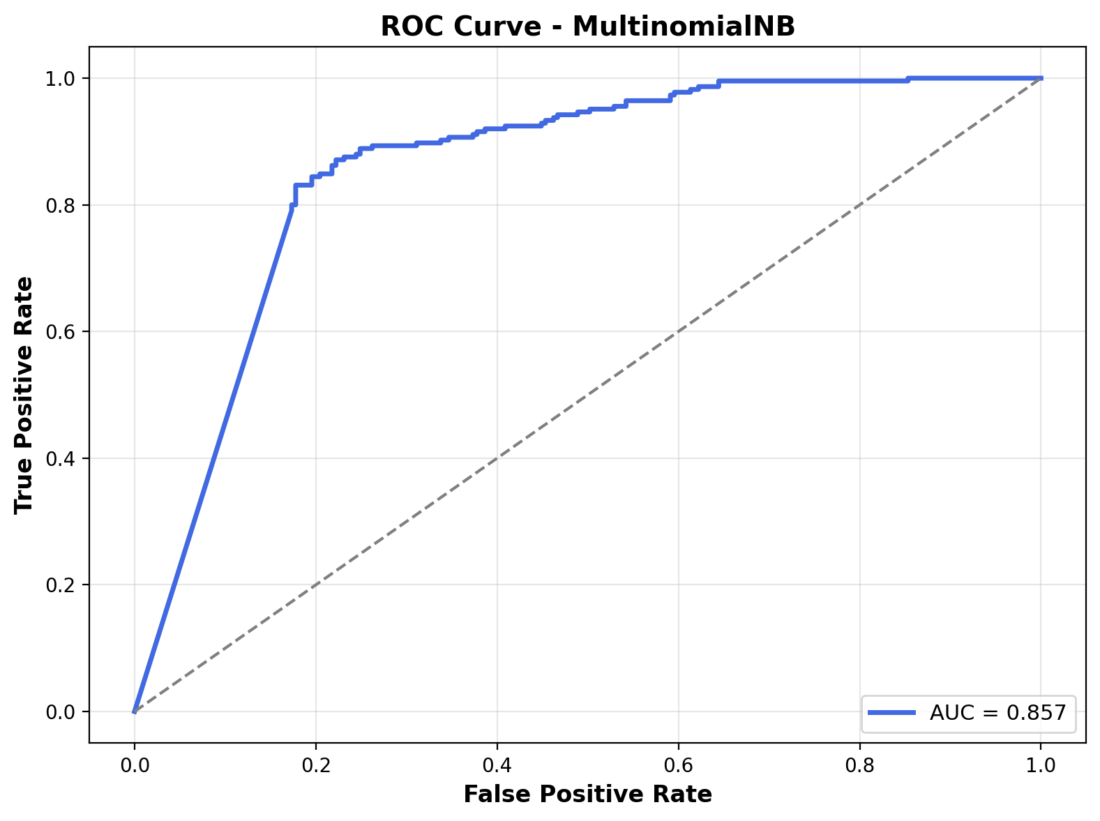
The ROC curve shows how the model balances sensitivity and specificity across different thresholds. The Area Under the Curve (AUC) is 0.857, which, while respectable, is lower than the 0.951 AUC of the logistic regression model. This suggests that the logistic regression classifier has a stronger ability to separate the two sound classes compared to Multinomial Naive Bayes.
Conclusion
Logistic Regression outperformed Multinomial Naive Bayes on the binary classification task involving sirens and fireworks. With an accuracy of 88.2% and an AUC of 0.951, the logistic model demonstrated stronger class separation and higher precision across the board. It achieved higher precision, recall, and F1-scores for both classes compared to the Multinomial Naive Bayes model, which reached an accuracy of 82.0% and AUC of 0.857.
While both models used the same discretized features, Logistic Regression benefited from its ability to model continuous probability boundaries, whereas Multinomial Naive Bayes relied on count-based assumptions. The results highlight that even with identical input representations, model choice can significantly impact classification performance; Logistic Regression consistently outperformed Multinomial Naive Bayes across every evaluation metric.
The full script to perform both Logistic Regression and Multinomial Naive Bayes classification, including preprocessing and visualizations, can be found here.