Supervised Learning (cont.)

Support Vector Machines

Overview

Support Vector Machines (SVMs) are powerful supervised learning algorithms used for classification, regression, and outlier detection. SVMs are particularly effective in high-dimensional spaces and cases where the number of dimensions exceeds the number of samples. The core idea behind SVMs is to find the optimal hyperplane that maximizes the margin between different classes in the feature space. This margin maximization gives SVMs strong generalization properties, making them less prone to overfitting compared to many other classifiers.

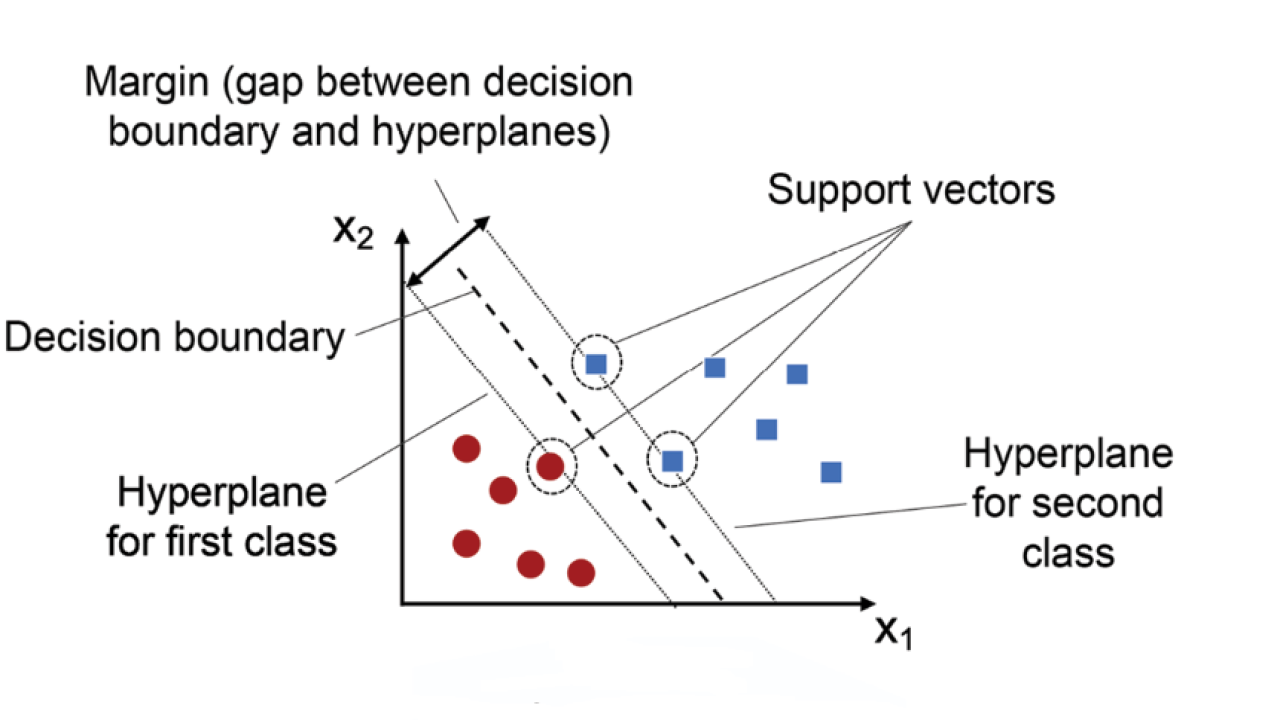
This illustration shows the fundamental concept of SVMs. The algorithm finds the hyperplane that maximizes the margin between classes. The margin is the distance between the hyperplane and the closest data points from each class, known as support vectors (circled). These support vectors are the only data points that determine the hyperplane's position, making SVMs robust to outliers far from the decision boundary.

Linear Separability and Hyperplanes

At their core, SVMs are linear classifiers that separate data points using a hyperplane. In a 2D space, this hyperplane is a straight line; in 3D, it's a flat plane; and in higher dimensions, it becomes an n-1 dimensional flat subspace. The decision function for an SVM is based on the position of a data point relative to this hyperplane, which is defined by the equation:

f(x) = w · x + b

Where w is the normal vector to the hyperplane, x is the input feature vector, and b is the bias term. The classification rule is simple: if f(x) ≥ 0, the point belongs to the positive class; otherwise, it belongs to the negative class.

What makes SVMs special is how they choose the optimal hyperplane among infinitely many possible separating hyperplanes. The SVM algorithm selects the hyperplane that maximizes the margin—the distance between the hyperplane and the closest data points from each class, called support vectors. This maximum margin strategy enhances the model's generalization ability to unseen data.

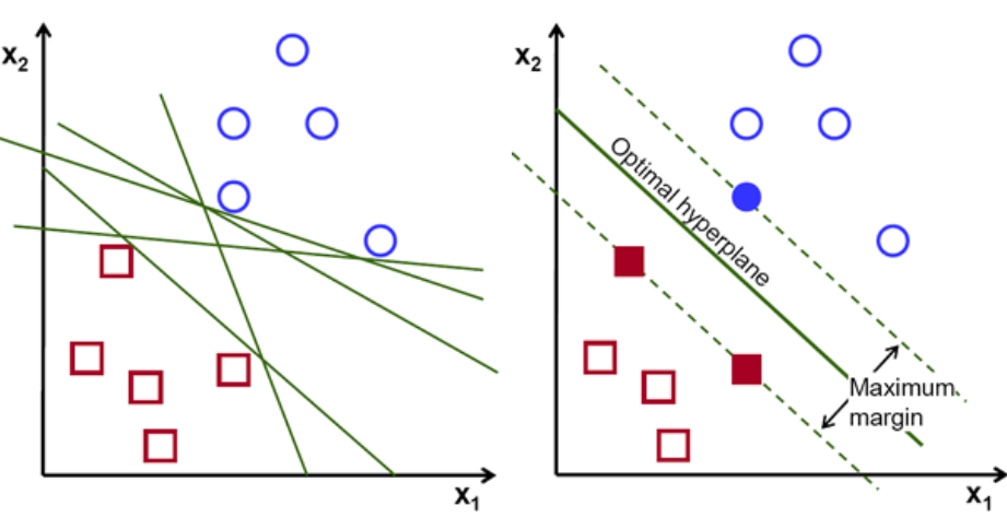
This image illustrates the concept of margin maximization in SVMs. The left panel shows multiple possible hyperplanes (green lines) that can separate the two classes (red squares and blue circles). The right panel highlights the optimal hyperplane (solid green line) which maximizes the margin between the classes. The margin boundaries (dashed green lines) pass through the support vectors (filled red squares and blue circle), which are the critical data points that define the decision boundary. By maximizing this margin, SVMs create more robust classification boundaries that generalize better to unseen data.

The Kernel Trick and Dot Products

While SVMs are inherently linear classifiers, they can effectively handle non-linear classification tasks through a mathematical technique called the kernel trick. The kernel trick allows SVMs to operate in an implicit higher-dimensional feature space without ever computing the coordinates of the data in that space.

The key insight is that the SVM algorithm only depends on inner products (dot products) between data points, not on the data points themselves. The dot product measures the similarity between two vectors and is calculated as:

x · y = Σ(x_i × y_i)

A kernel function K(x, y) effectively computes the dot product in a higher-dimensional space without explicitly transforming the data:

K(x, y) = φ(x) · φ(y)

Where φ(x) represents the transformation to the higher-dimensional space. By substituting kernel functions for dot products, SVMs can learn non-linear decision boundaries in the original feature space.

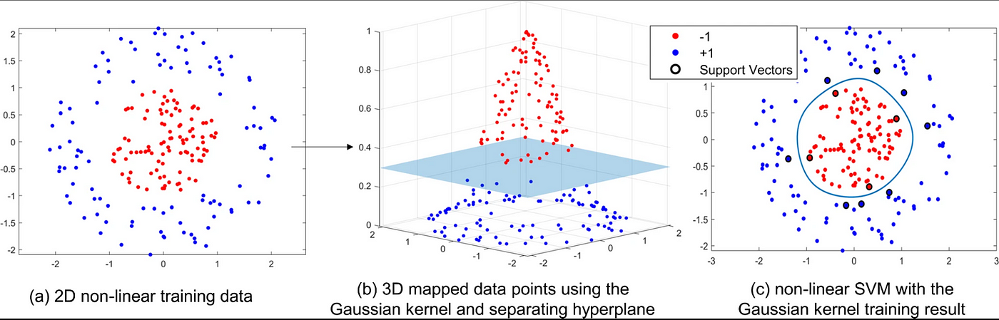
This visualization demonstrates the kernel trick. The left side shows data that's not linearly separable in 2D space. The middle shows how these points can be mapped to a higher-dimensional space (3D in this example) where they become linearly separable. The right side shows the resulting nonlinear decision boundary when projected back to the original 2D space.

Example: Polynomial Kernel Transformation

To illustrate how a kernel implicitly maps data to a higher-dimensional space, consider a 2D point (x₁, x₂) and a polynomial kernel with degree d = 2 and coefficient r = 1:

K(x, y) = (x · y + r)^d = (x₁y₁ + x₂y₂ + 1)^2

When expanded, this becomes:

K(x, y) = (x₁y₁ + x₂y₂ + 1)^2 = (x₁y₁)^2 + (x₂y₂)^2 + 2(x₁y₁)(x₂y₂) + 2x₁y₁ + 2x₂y₂ + 1

This expansion corresponds to the dot product in a 6-dimensional space where the original 2D point (x₁, x₂) is mapped to:

φ(x) = (x₁², x₂², √2x₁x₂, √2x₁, √2x₂, 1)

The beauty of the kernel trick is that this transformation is never explicitly computed. Instead, the kernel function directly calculates what the dot product would be in this higher-dimensional space. This makes SVMs computationally efficient even when the implicit feature space has very high or even infinite dimensions, as with the Radial Basis Function (RBF) kernel.

Common Kernel Functions

Common kernels include linear, polynomial, radial basis function (RBF), and sigmoid. Each kernel transforms the input space differently to enable the SVM to find an optimal separating boundary. The linear kernel is best suited for linearly separable data, while the polynomial and RBF kernels allow the model to capture complex, non-linear relationships. The choice of kernel has a significant impact on the model’s ability to generalize to unseen data.

Linear Kernel

K(x, y) = x · y

The simplest kernel, equivalent to no transformation. Effective when the data is already linearly separable. Computationally efficient and interpretable, as the original feature space is preserved.

Polynomial Kernel

K(x, y) = (γx · y + r)^d

Creates polynomial combinations of features up to degree d. The parameters γ (gamma), r (coefficient), and d (degree) control the flexibility of the decision boundary. Useful for problems where feature interactions matter.

RBF Kernel

K(x, y) = exp(-γ||x - y||²)

The Radial Basis Function (Gaussian) kernel measures similarity based on distance between points. Creates complex, localized decision boundaries. The parameter γ controls the influence radius of each support vector.

Sigmoid Kernel

K(x, y) = tanh(γx · y + r)

Inspired by neural networks, this kernel applies a hyperbolic tangent transformation. Its effectiveness depends heavily on proper hyperparameter tuning. Less commonly used than RBF or polynomial kernels.

SVM Classification of Audio Data

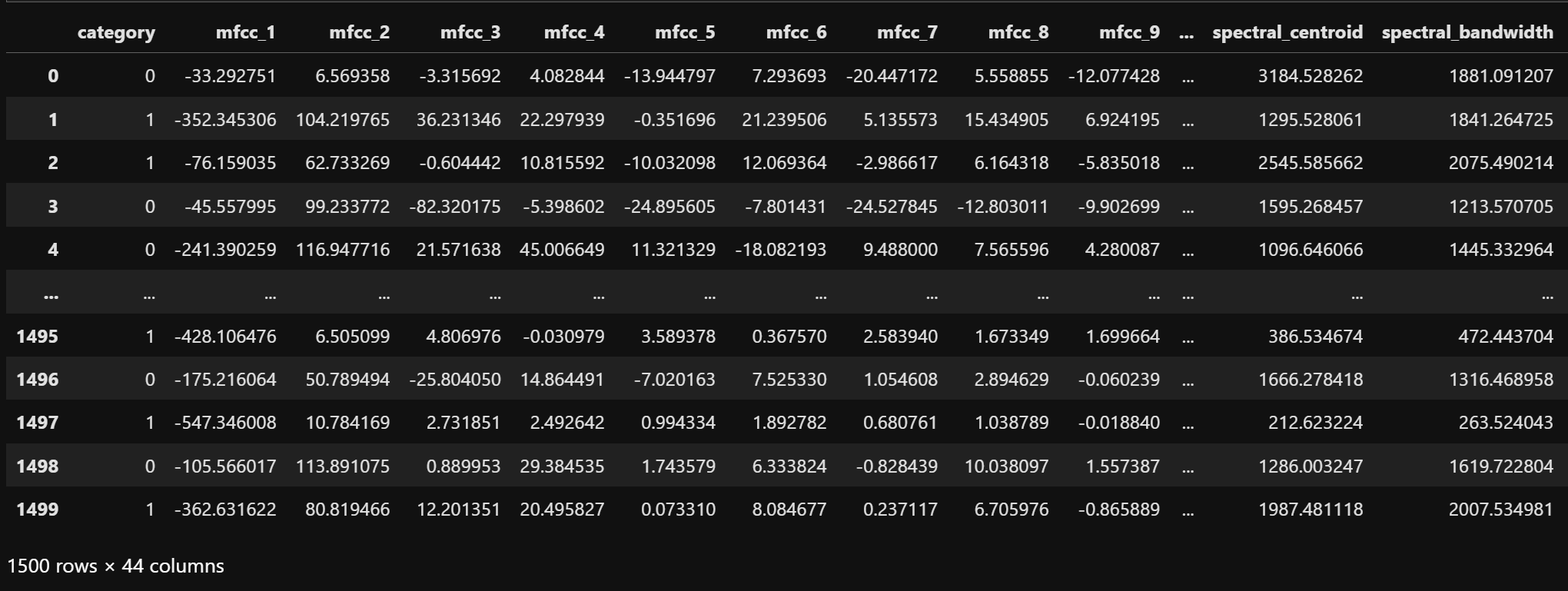
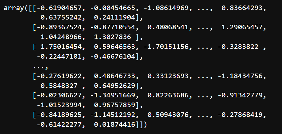
To apply SVM to audio classification, a dataset consisting of audio features from two categories is selected: "laughter" and "footsteps". This binary classification task provides a clear benchmark for evaluating different SVM configurations. The raw dataset is shown below.

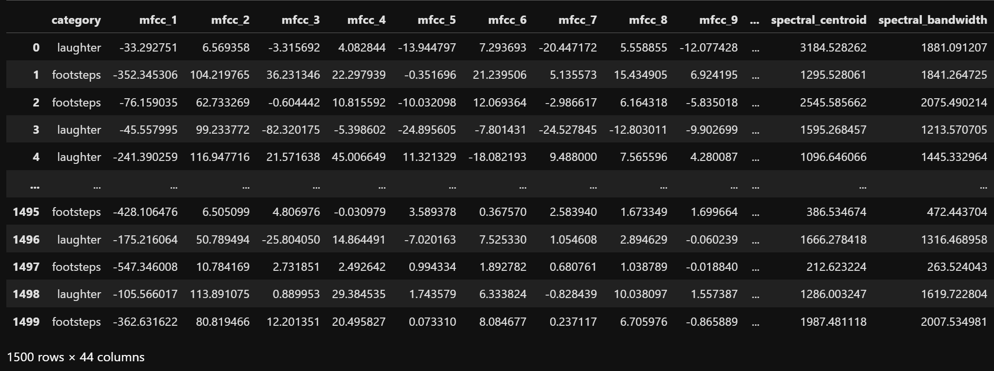
The dataset contains extracted audio features for both "laughter" and "footsteps" categories. Each row represents one audio sample, with columns corresponding to various audio features like spectral contrast, MFCCs, chroma, and other acoustic descriptors.

For the classification task, the categories are encoded as binary values: "laughter" as 0 and "footsteps" as 1. This encoded dataset serves as the foundation for the SVM models. The encoded dataset is shown below.

The dataset after binary encoding of categories. The "category" column now contains numeric values (0 for "laughter", 1 for "footsteps") suitable for machine learning algorithms.

All supervised learning methods require splitting data into training and testing sets to evaluate model performance objectively. This ensures that models are evaluated on data they haven't seen during training, providing a reliable estimate of how well they'll perform on new, unseen data. The dataset is split into training (70%) and testing (30%) sets using stratified sampling to maintain class distribution. The training and testing sets are shown below.

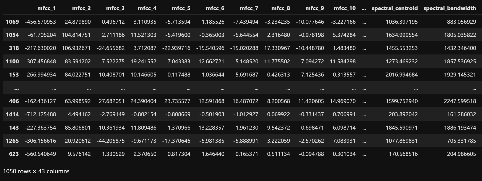
The training dataset contains 70% of the original samples, maintaining the same class distribution. This set is used to train the SVM models.

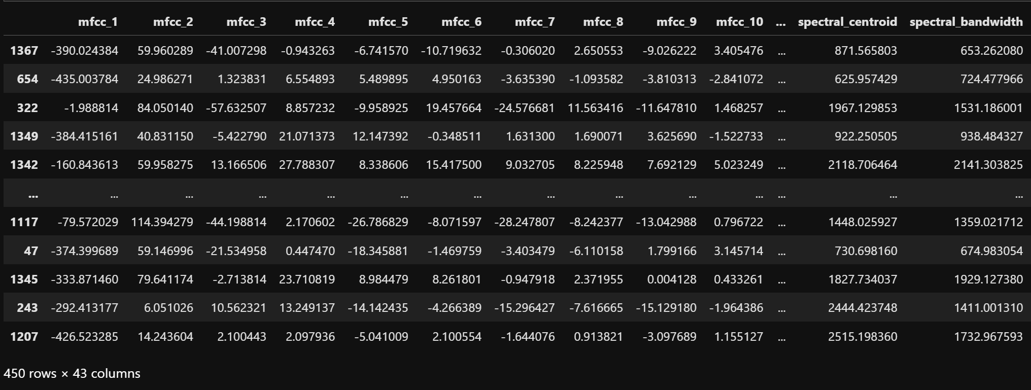
The testing dataset contains the remaining 30% of samples and is used to evaluate model performance on unseen data.

SVMs are sensitive to feature scaling, so proper preprocessing is essential. The features are standardized using StandardScaler, which transforms each feature to have zero mean and unit variance. This preprocessing is crucial for SVM performance, as the algorithm's distance calculations are directly affected by feature magnitudes. All features are standardized to have zero mean and unit variance, which helps prevent features with larger scales from dominating the model. The scaled training and testing sets are shown below.

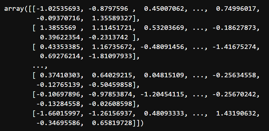
This images depicts the scaled training data. The features are scaled to a standard normal distribution with mean=0 and variance=1.

This images depicts the scaled testing data. The features are scaled to a standard normal distribution using parameters calculated on the training data.

Implementing SVM with Different Kernels

Three different SVM kernels are implemented to explore their effectiveness on audio classification:

Linear Kernel: The simplest form of SVM, creating straight-line decision boundaries in the original feature space.
RBF Kernel (Radial Basis Function): A flexible, non-linear kernel that can capture complex relationships through implicitly mapping data to an infinite-dimensional space.
Polynomial Kernel (degree=3): Creates feature combinations up to the specified degree, allowing for curved decision boundaries.

For each kernel type, three different regularization parameter (C) values are tested: 0.5, 10, and 100. The C parameter controls the trade-off between achieving a smooth decision boundary and correctly classifying training points:

C=0.5: A smaller value that prioritizes a smoother decision boundary, potentially at the cost of misclassifying more training points.
C=10: A moderate value balancing between decision boundary smoothness and training accuracy.
C=100: A larger value that emphasizes correctly classifying training points, potentially at the cost of overfitting.

The implementation uses scikit-learn's SVC (Support Vector Classification) with probability estimates enabled for ROC curve analysis. Each model is evaluated on the test set using multiple metrics including accuracy, precision, recall, F1-score, confusion matrix, and area under the ROC curve (AUC).

Additionally, for visualization purposes, the high-dimensional feature space is reduced to 2D using Principal Component Analysis (PCA). This allows plotting of the decision boundaries in a way that human eyes can interpret, though it's important to note that the actual classification happens in the original feature space.

SVM with Linear Kernel and C=0.5

The linear kernel creates a straight-line decision boundary with minimal complexity. With C=0.5, this configuration prioritizes a smoother boundary over perfect classification of training points, establishing a baseline against which more complex kernel functions can be compared.

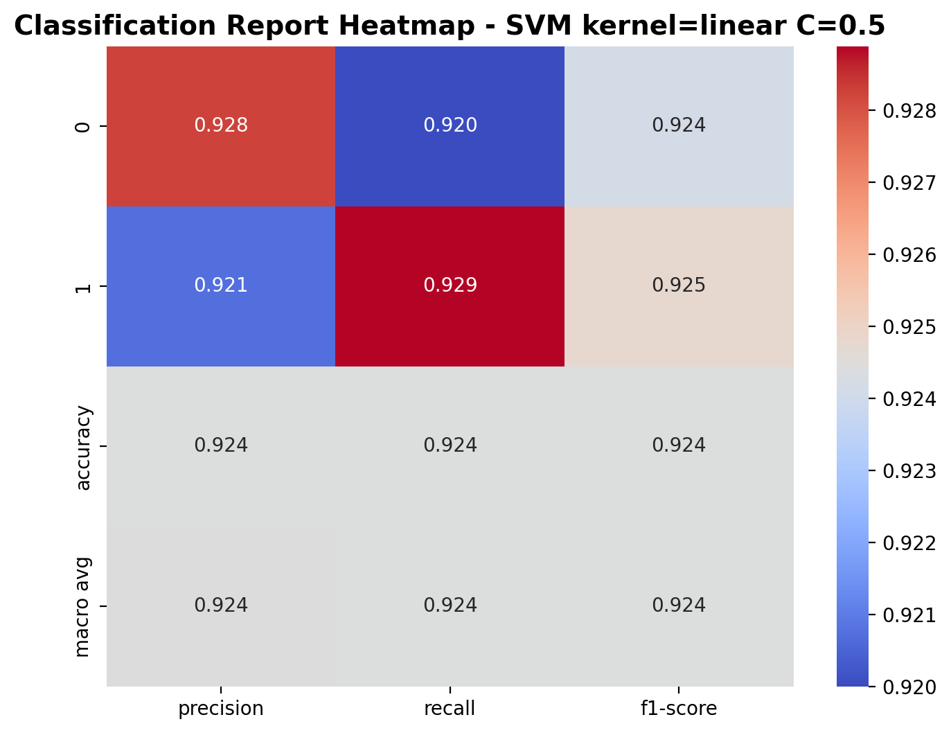
Classification Report - Linear Kernel C=0.5

The classification report shows the performance metrics for the linear kernel SVM with C=0.5. For class 0 (laughter), the model achieved a precision of 0.928, recall of 0.920, and F1-score of 0.924. For class 1 (footsteps), the precision was 0.921, recall was 0.929, and F1-score was 0.925. The overall accuracy is 92.4%, with similar macro-average metrics, indicating balanced performance across both classes.

The confusion matrix provides a detailed breakdown of predictions. The model correctly classified 207 laughter samples and 209 footstep samples, while misclassifying 18 laughter samples as footsteps and 16 footstep samples as laughter.

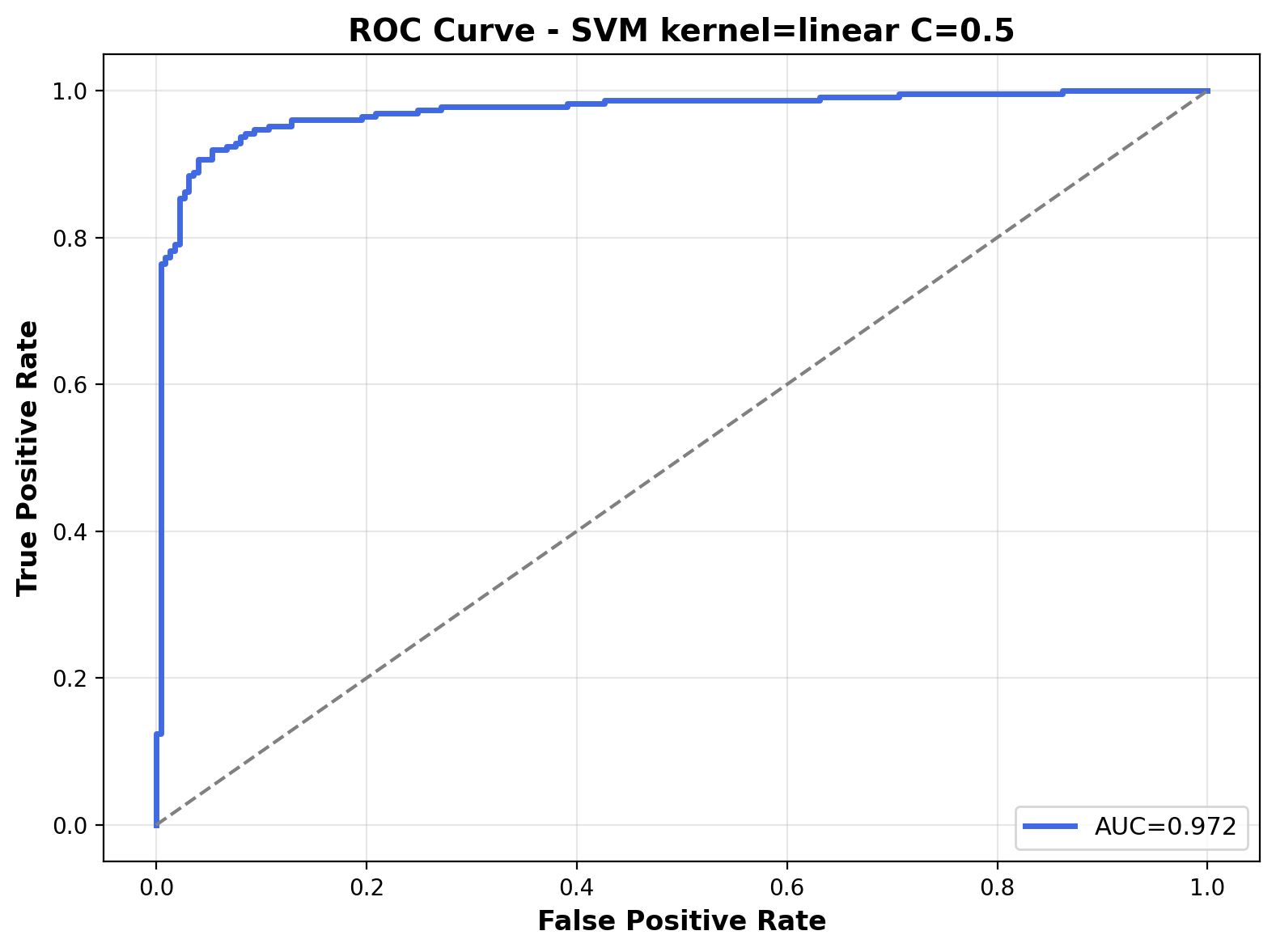
The ROC curve illustrates the model's performance across different classification thresholds. The Area Under the Curve (AUC) is 0.972, indicating very strong classification performance. The curve's proximity to the top-left corner reflects the model's ability to differentiate between the two audio classes.

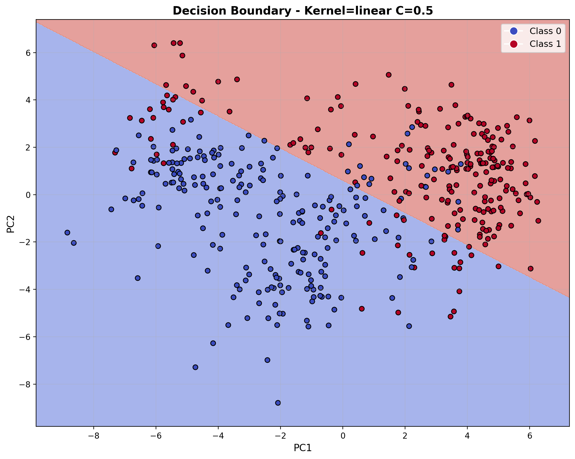
This visualization shows the decision boundary of the linear kernel SVM in a 2D space created by PCA. The linear kernel creates a straight-line boundary (in the reduced dimension space) separating the two classes. While the boundary appears clean, there are still some misclassifications in regions where the classes overlap. The regularization parameter C=0.5 results in a slightly smoother boundary that doesn't try to perfectly separate all training points.

Linear Kernel with C=10

With an increased C value of 10, this linear kernel model places greater emphasis on correctly classifying training points while still maintaining a straight-line decision boundary. This medium regularization strength allows the model to better fit the training data while still providing reasonable generalization to unseen examples.

Classification Report - Linear Kernel C=10

With C=10, the linear kernel SVM shows great performance. For class 0 (laughter), precision is 0.937, recall is 0.924, and F1-score is 0.931. For class 1 (footsteps), precision is 0.925, recall is 0.938, and F1-score is 0.932. The overall accuracy has increased to 93.1%, showing that the higher C value allows the model to better fit the training data while still generalizing well to the test set.

The confusion matrix shows 208 correctly classified laughter samples and 211 correctly classified footstep samples. Misclassifications have decreased to 17 laughter samples predicted as footsteps and 14 footstep samples predicted as laughter.

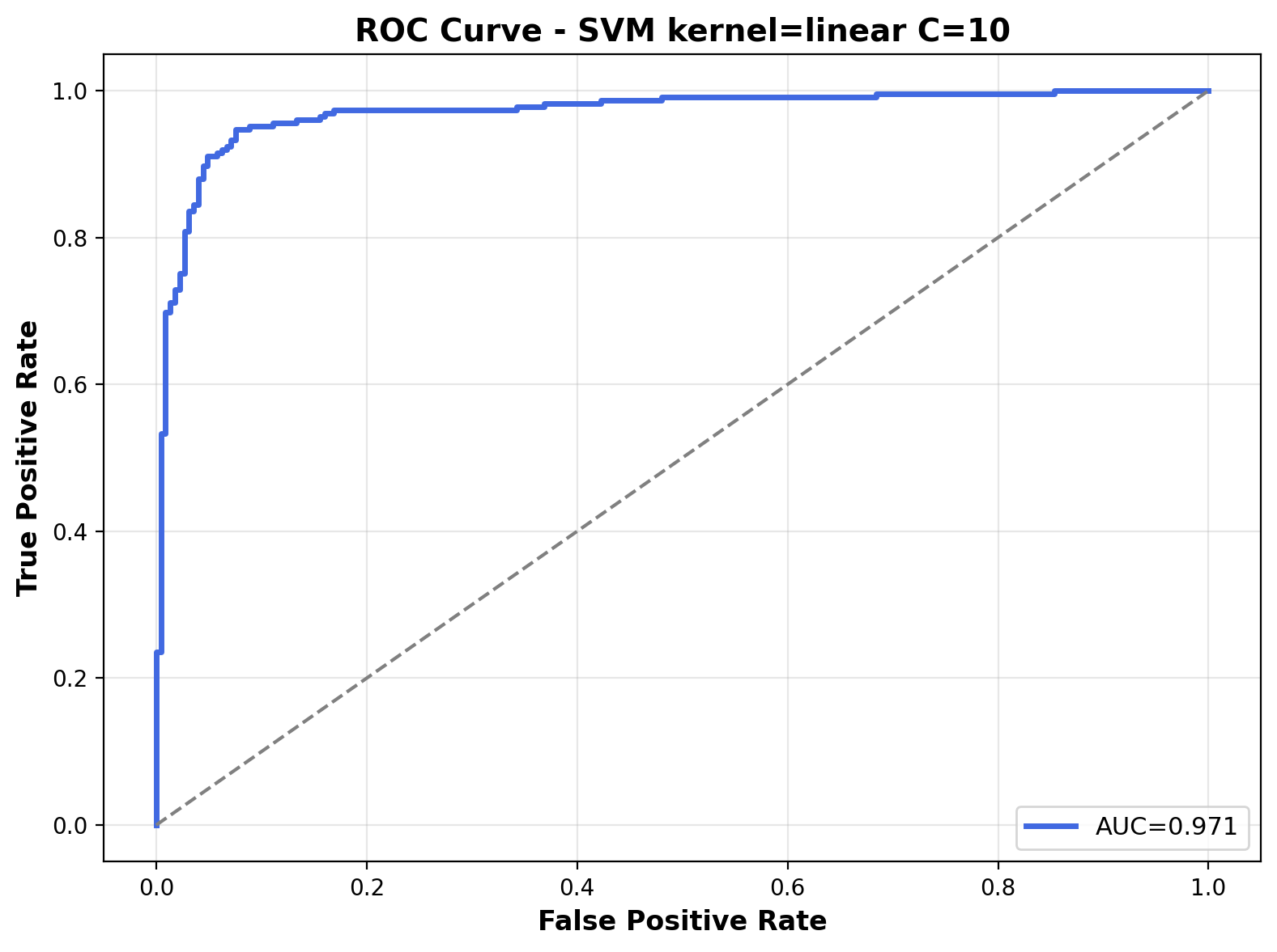
The ROC curve illustrates the model's performance across different classification thresholds. The Area Under the Curve (AUC) is 0.971, indicating strong classification performance. The curve's proximity to the top-left corner reflects the model's ability to differentiate between the two audio classes with great confidence.

The decision boundary visualization shows the linear separator in the reduced 2D feature space created by PCA. The boundary creates a clear division between the two audio classes, with most points correctly classified on their respective sides. As characteristic of the linear kernel, the boundary forms a straight line through the feature space, attempting to maximize the margin while respecting the C=10 regularization parameter.

Linear Kernel with C=100

At C=100, the linear kernel model strongly prioritizes correct classification of training points over boundary smoothness. This high regularization parameter pushes the model to minimize training errors, potentially at the cost of generalization. Despite the high C value, the decision boundary remains linear in nature.

Classification Report - Linear Kernel C=100

With C=100, the linear kernel SVM shows great performance again. For class 0 (laughter), precision is 0.941, recall is 0.916, and F1-score is 0.928. For class 1 (footsteps), precision is 0.918, recall is 0.942, and F1-score is 0.930. The overall accuracy of the model is 92.9%, indicating strong classification performance for this binary audio task.

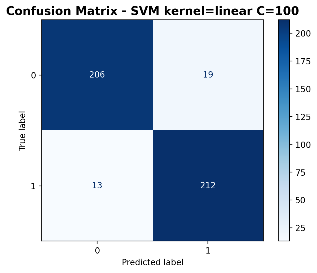
The confusion matrix shows 206 correctly classified laughter samples and 212 correctly classified footstep samples. Misclassifications include 19 laughter samples predicted as footsteps and 13 footstep samples predicted as laughter.

The ROC curve illustrates the model's performance across different classification thresholds. The Area Under the Curve (AUC) is 0.969, indicating strong classification performance. The curve's proximity to the top-left corner reflects the model's ability to differentiate between the two audio classes with great confidence.

The decision boundary visualization for the linear kernel with C=100 shows a straight-line separator dividing the feature space in the reduced PCA dimensions. The boundary creates a clear division between the two audio classes, with the majority of points properly classified on their respective sides. As expected from a linear kernel, the decision boundary remains a straight line regardless of the regularization strength, creating a simple but effective separation for this binary audio classification task.

RBF Kernel with C=0.5

The Radial Basis Function (RBF) kernel enables non-linear decision boundaries by implicitly mapping data to an infinite-dimensional space. With C=0.5, the model creates smooth, curved boundaries that can better adapt to the underlying structure of audio data while avoiding overfitting to noise or outliers.

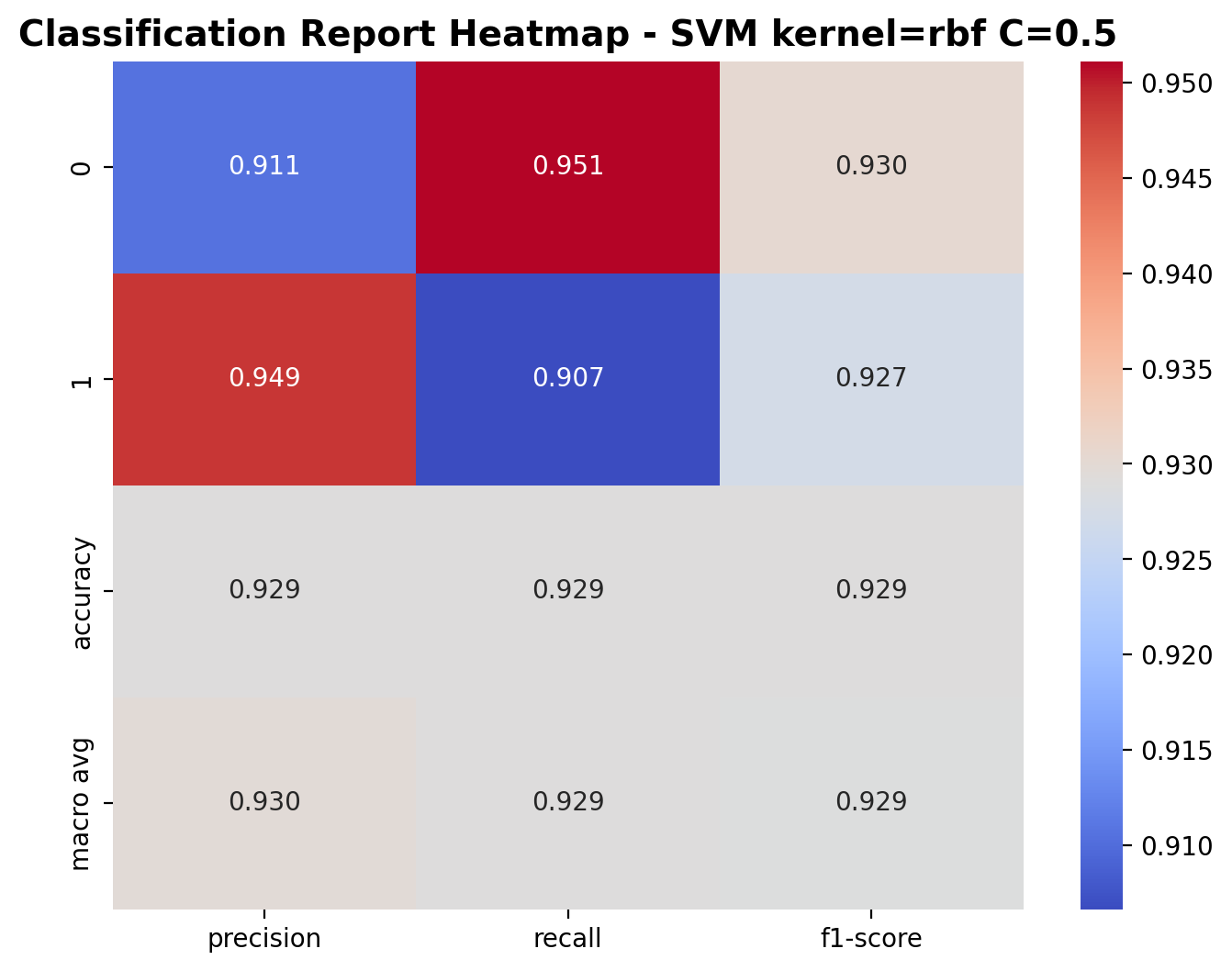
Classification Report - RBF Kernel C=0.5

The RBF kernel with C=0.5 shows impressive performance as well. For class 0 (laughter), precision is 0.911, recall is 0.951, and F1-score is 0.930. For class 1 (footsteps), precision is 0.949, recall is 0.907, and F1-score is 0.927. The overall accuracy is 92.9%, demonstrating the RBF kernel's ability to capture relationships in the audio feature space.

The confusion matrix shows 214 correctly classified laughter samples and 204 correctly classified footstep samples. Misclassifications include 11 laughter samples predicted as footsteps and 21 footstep samples predicted as laughter.

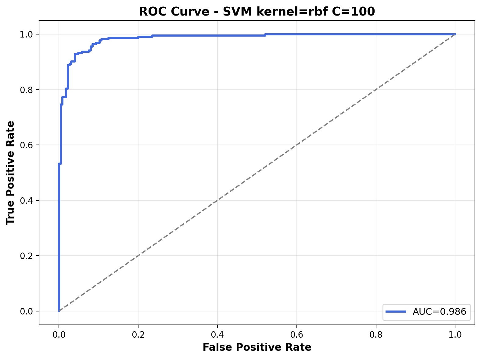
The ROC curve shows exceptional discriminative power with an AUC of 0.986. The curve hugs the top-left corner indicating the RBF kernel's ability to distinguish between the two audio classes even with a relatively conservative regularization parameter.

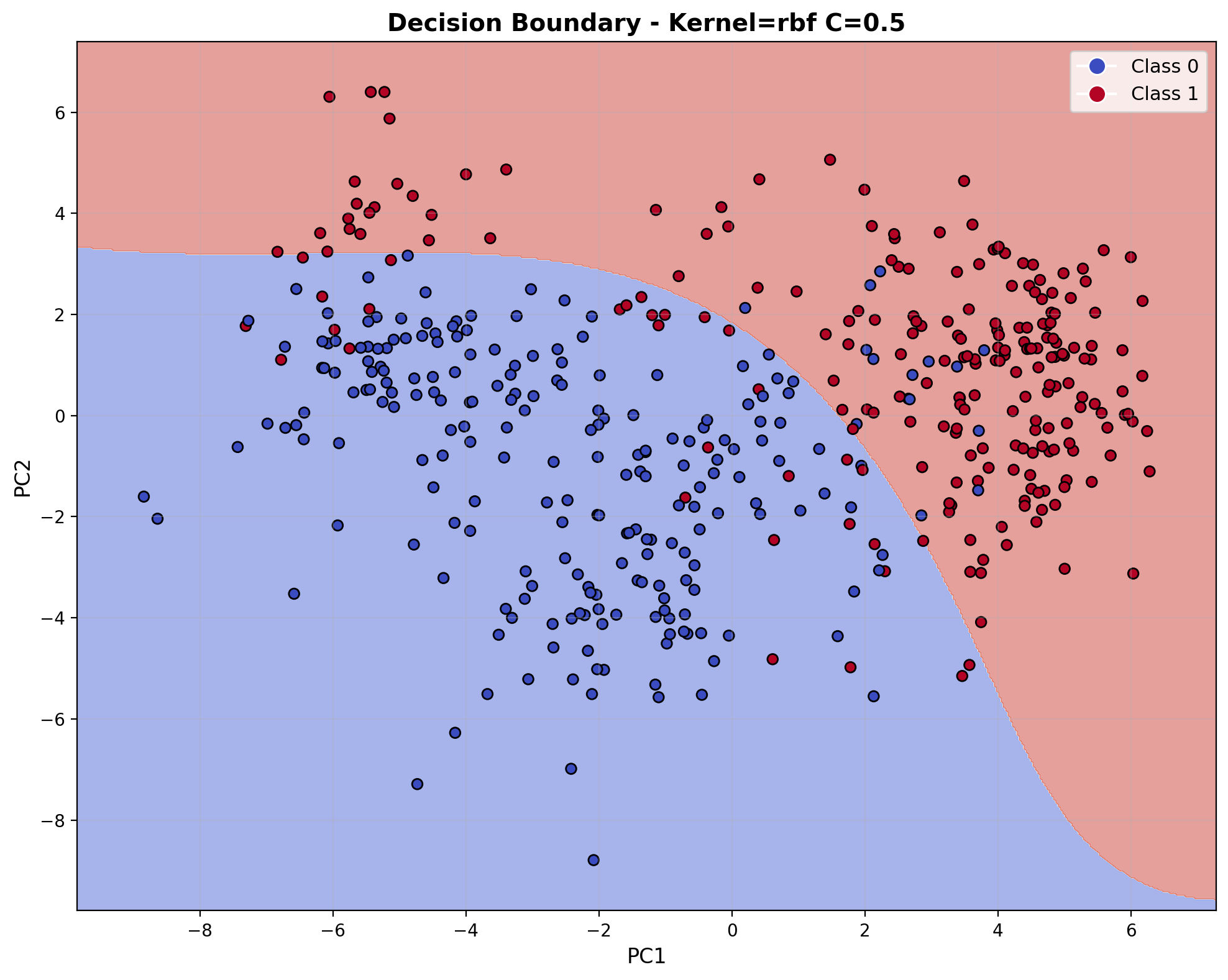
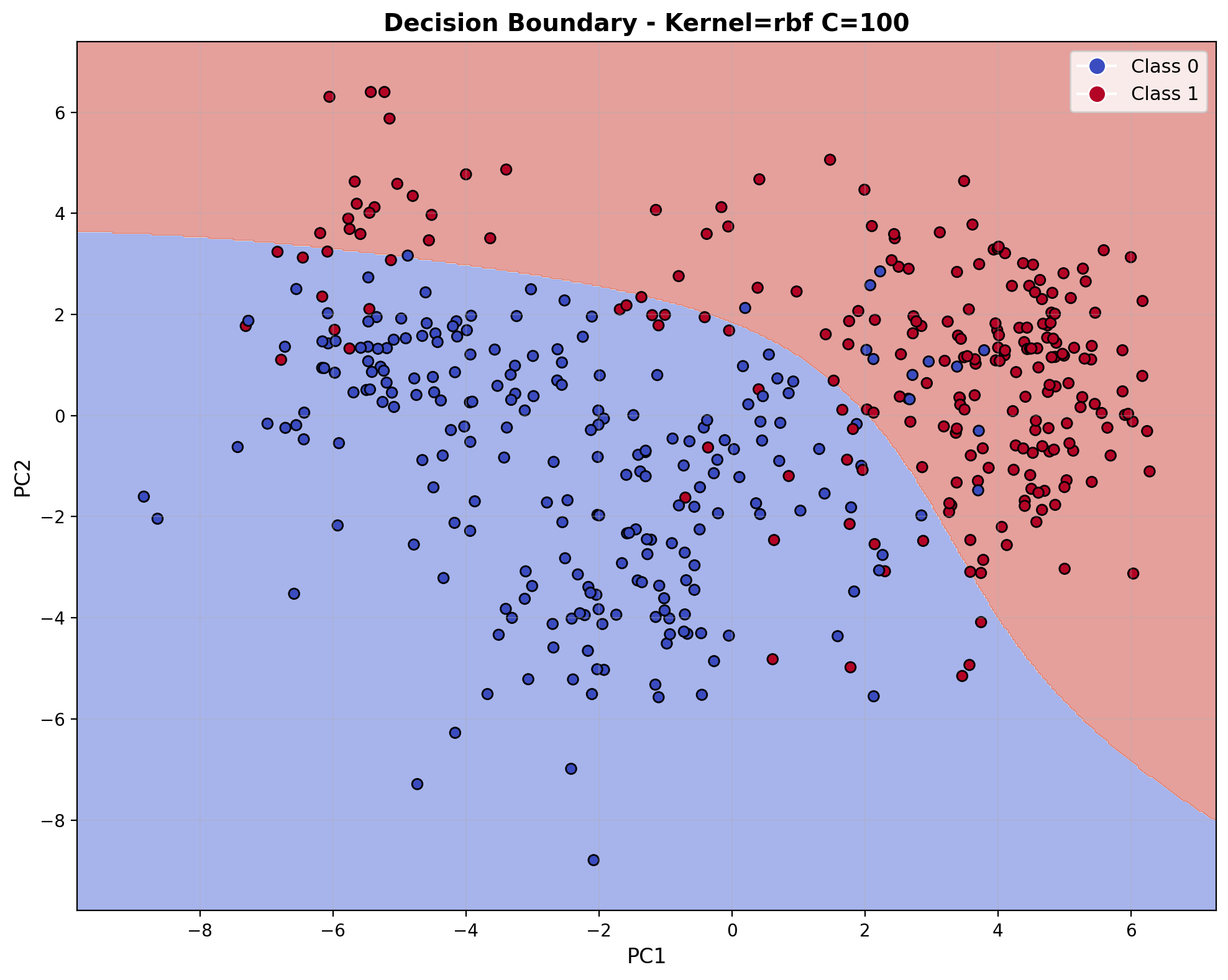
The decision boundary visualization reveals a fundamentally different shape compared to the linear models. The RBF kernel creates curved, non-linear boundaries that can enclose regions and better adapt to the data distribution. With C=0.5, the boundary remains relatively smooth while still capturing the underlying non-linear structure of the audio feature space.

RBF Kernel with C=10

The RBF kernel with C=10 represents a balanced configuration that permits more complex decision boundaries while still maintaining good generalization. This setting allows the model to create more intricate decision regions that better capture the non-linear relationships present in audio feature spaces.

With C=10, the RBF kernel SVM improves its performance significantly. For class 0 (laughter), precision is 0.934, recall is 0.951, and F1-score is 0.943. For class 1 (footsteps), precision is 0.950, recall is 0.933, and F1-score is 0.942. The overall accuracy reaches an impressive 94.2%, showing that the increased regularization parameter allows the model to better adapt to the complex patterns in audio features.

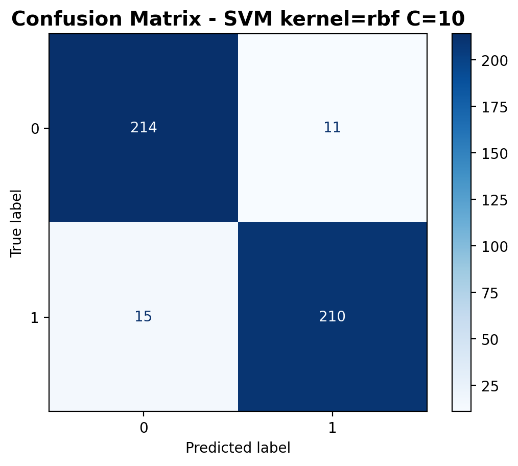
The confusion matrix shows improvement with 214 correctly classified laughter samples and 210 correctly classified footstep samples. Misclassifications have decreased to 11 laughter samples predicted as footsteps and 15 footstep samples predicted as laughter.

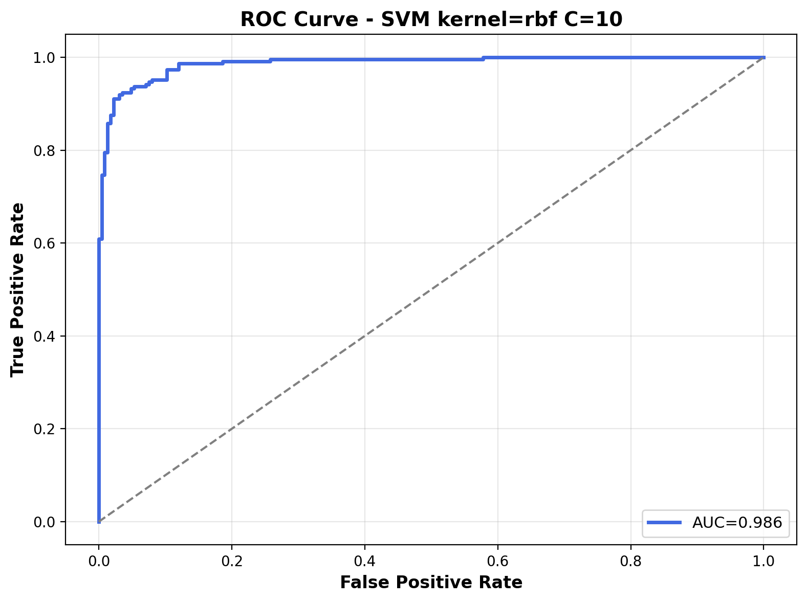
The ROC curve shows exceptional performance with an AUC of 0.986. The curve hugs the top-left corner, indicating the RBF kernel with C=10 achieves excellent separation between the two audio classes across various probability thresholds.

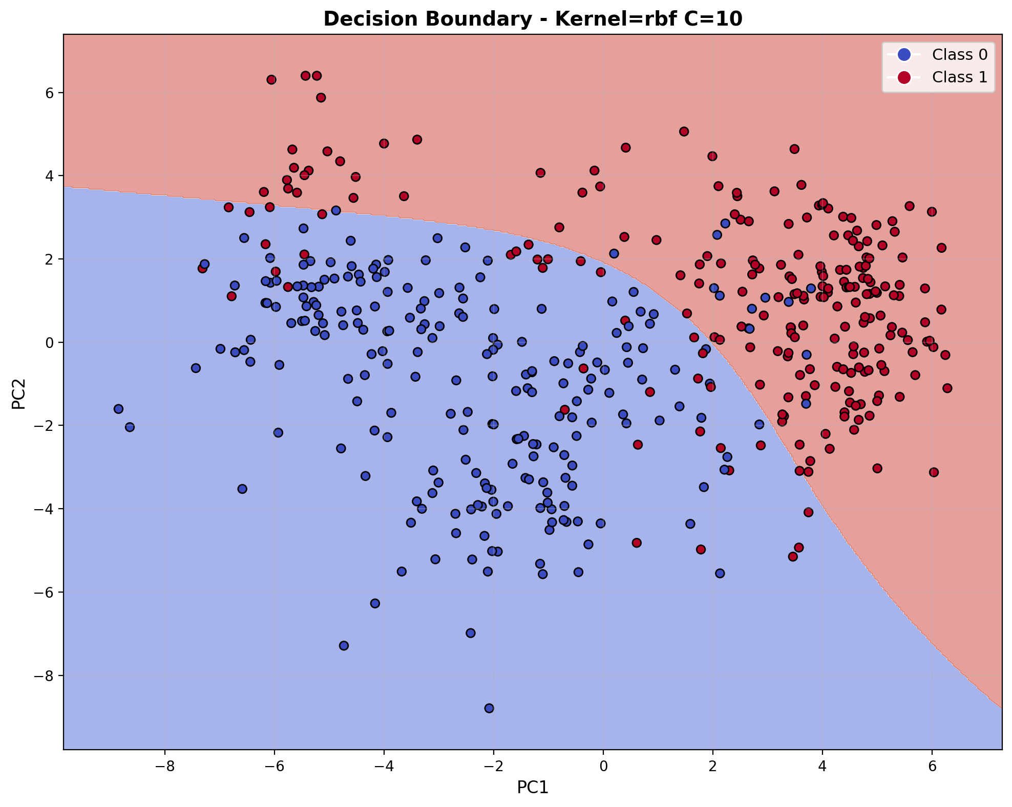
The decision boundary visualization for the RBF kernel with C=10 reveals the model's ability to create curved, non-linear separations in the feature space. The boundary forms complex regions that adapt to the data distribution, creating localized areas of classification rather than a single straight line. This flexibility allows the RBF kernel to capture the nuanced acoustic patterns that differentiate between laughter and footstep sounds in the audio feature space.

RBF Kernel with C=100

At C=100, the RBF kernel model generates highly flexible decision boundaries that can closely fit the training data. This configuration allows the model to create complex, localized regions that precisely separate audio classes, capturing subtle patterns in the feature space that simpler models might miss.

Classification Report - RBF Kernel C=100

With C=100, the RBF kernel SVM performs similarly. For class 0 (laughter), precision is 0.927, recall is 0.960, and F1-score is 0.943. For class 1 (footsteps), precision is 0.959, recall is 0.924, and F1-score is 0.941. The overall accuracy stays 94.2%, demonstrating that further increasing the regularization parameter provides minimal benefits for this audio classification task.

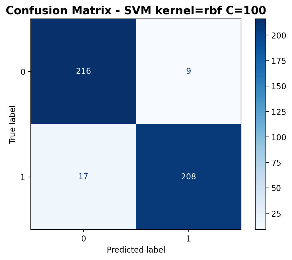
The confusion matrix shows similar performance with 216 correctly classified laughter samples and 208 correctly classified footstep samples. Misclassifications include 9 laughter samples predicted as footsteps and 17 footstep samples predicted as laughter.

The ROC curve shows the same outstanding performance with an AUC of 0.986. The curve hugs the top-left corner, indicating the RBF kernel with C=10 achieves excellent separation between the two audio classes across various probability thresholds.

The decision boundary visualization for the RBF kernel with C=100 reveals the model's ability to create curved, non-linear separations in the feature space. The boundary forms complex regions that adapt to the data distribution, creating localized areas of classification rather than a single straight line. This flexibility allows the RBF kernel to capture the nuanced acoustic patterns that differentiate between laughter and footstep sounds in the audio feature space.

Polynomial Kernel with C=0.5

The polynomial kernel (degree=3) creates curved decision boundaries by modeling feature interactions up to the specified degree. With C=0.5, the model maintains relatively smooth boundaries while capturing non-linear relationships, offering a middle ground between the rigidity of linear kernels and the flexibility of RBF kernels.

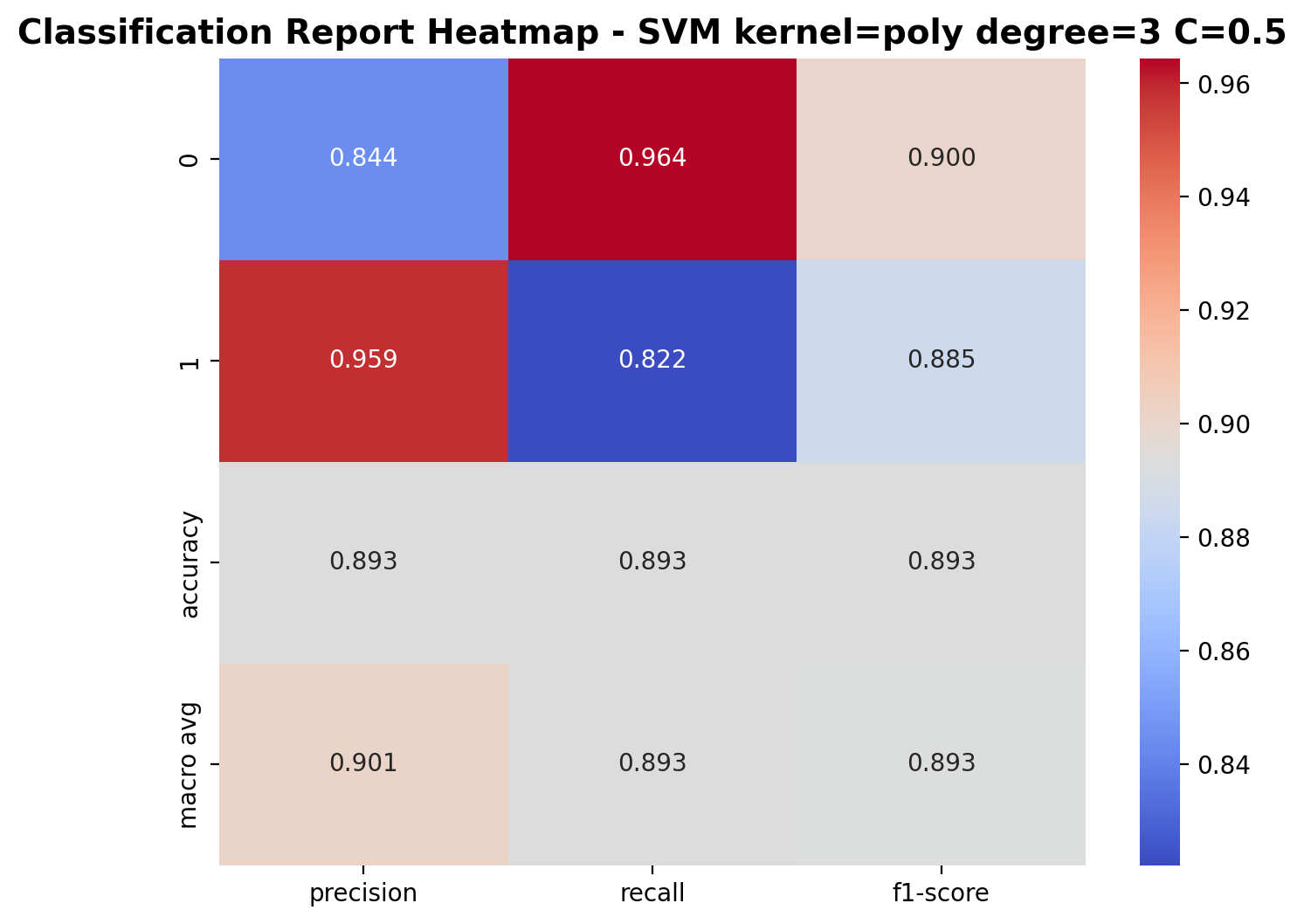
Classification Report - Polynomial Kernel C=0.5

The polynomial kernel (degree=3) with C=0.5 demonstrates decent performance. For class 0 (laughter), precision is 0.844, recall is 0.964, and F1-score is 0.900. For class 1 (footsteps), precision is 0.959, recall is 0.822, and F1-score is 0.885. The overall accuracy is 89.3%, demonstrating polynomial kernel's ability to capture patterns in the audio data.

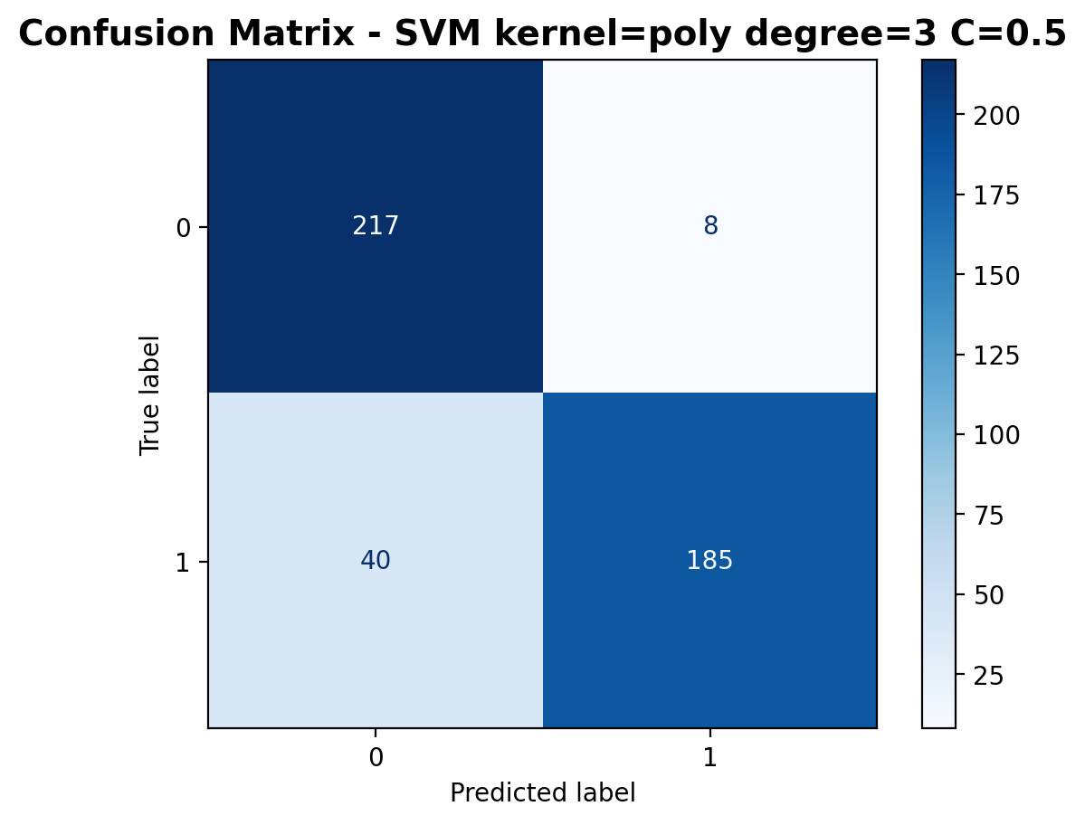
Confusion Matrix - Polynomial Kernel C=0.5

The confusion matrix shows 217 correctly classified laughter samples and 185 correctly classified footstep samples. Misclassifications include 8 laughter samples predicted as footsteps and 40 footstep samples predicted as laughter.

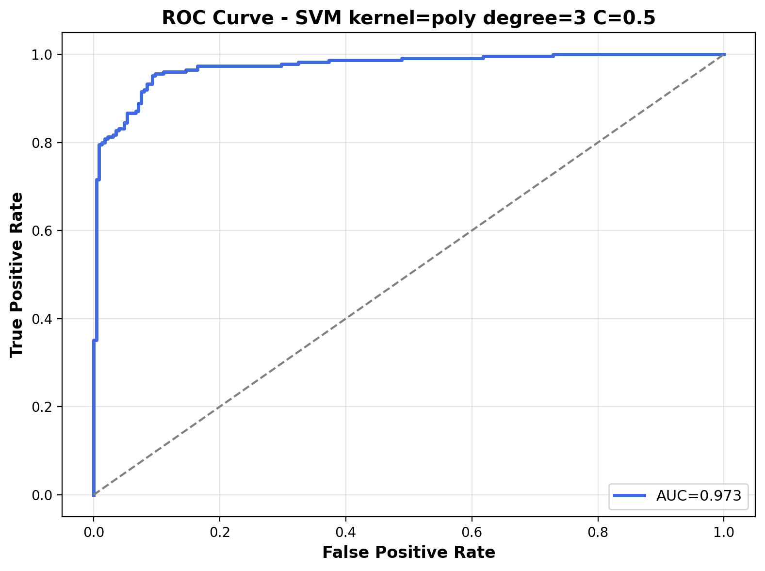
The ROC curve shows strong discriminative ability with an AUC of 0.973. It demonstrates the polynomial kernel's ability to separate the audio classes, particularly with this moderate regularization parameter.

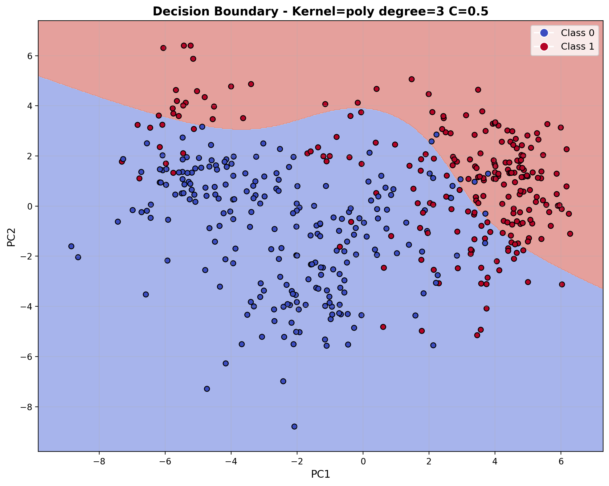
Decision Boundary - Polynomial Kernel C=0.5

The decision boundary visualization shows curved, polynomial-shaped boundaries that are more flexible than linear boundaries but less localized than RBF boundaries. With C=0.5, the boundary maintains a smooth, flowing shape that captures the general trend in the data while avoiding overly complex fits to individual points.

Polynomial Kernel with C=10

With C=10, the polynomial kernel model (degree=3) strikes a balance between boundary complexity and generalization ability. This configuration allows for more pronounced curves and loops in the decision boundary, better accounting for the polynomial relationships between audio features.

Classification Report - Polynomial Kernel C=10

With C=10, the polynomial kernel SVM shows improved performance. For class 0 (laughter), precision is 0.884, recall is 0.947, and F1-score is 0.914. For class 1 (footsteps), precision is 0.943, recall is 0.876, and F1-score is 0.908. The overall accuracy increases to 91.1%, demonstrating that a higher regularization parameter allows the polynomial kernel to better capture the complex patterns in audio features.

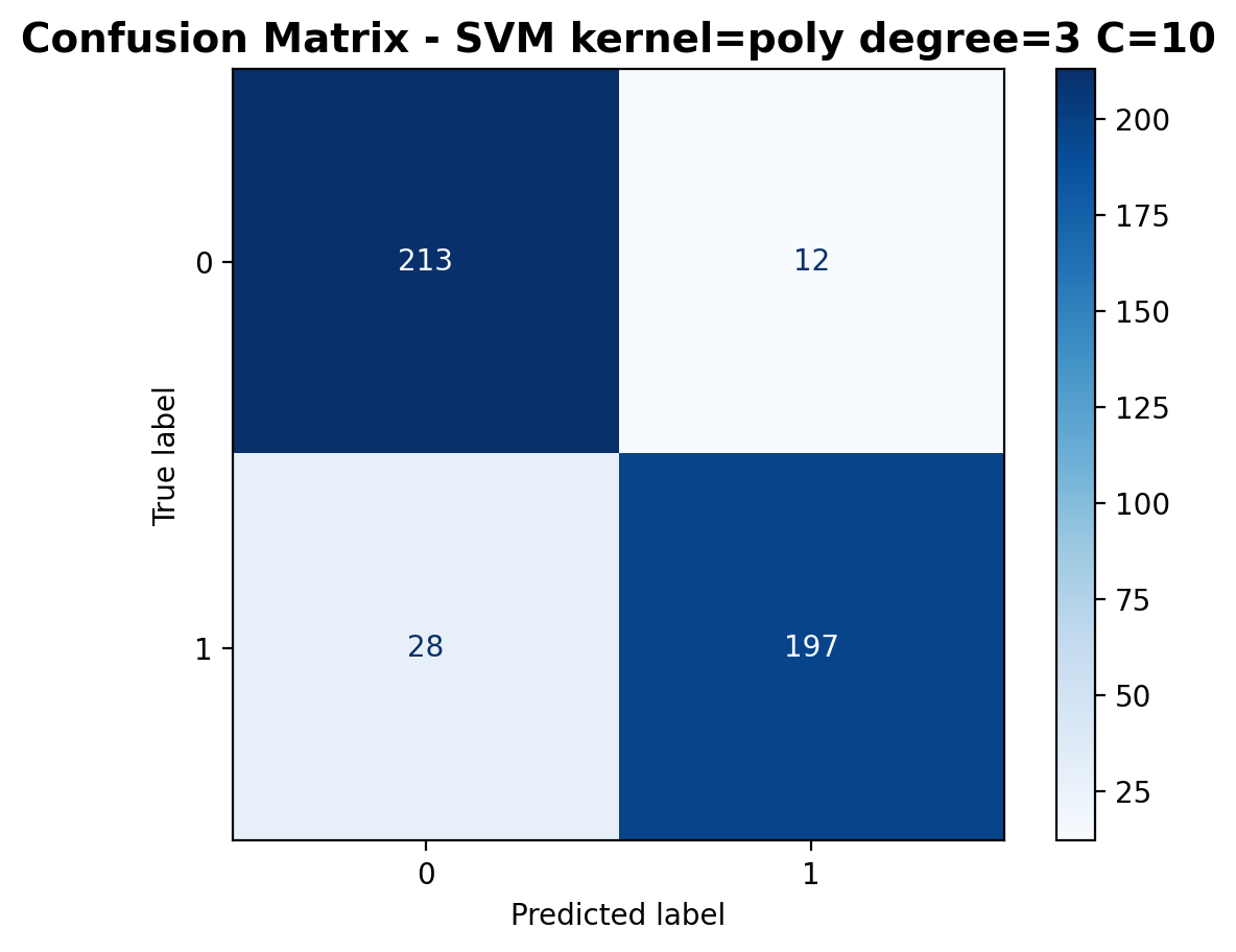
Confusion Matrix - Polynomial Kernel C=10

The confusion matrix shows 213 correctly classified laughter samples and 197 correctly classified footstep samples. Misclassifications have decreased to 28 laughter samples predicted as footsteps and 12 footstep samples predicted as laughter.

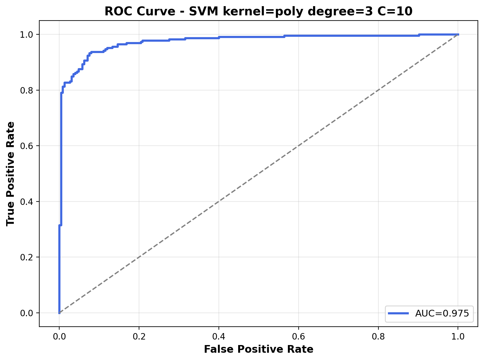
The ROC curve shows solid performance with an AUC of 0.975. The curve approaches the top-left corne, indicating that the polynomial kernel with C=10 achieves excellent separation between the two audio classes across various probability thresholds.

Decision Boundary - Polynomial Kernel C=10

The decision boundary visualization for the polynomial kernel (degree=3) with C=10 displays characteristic curved shapes with smooth transitions throughout the feature space. The boundary forms polynomial curves that separate the audio classes with moderate complexity, creating rounded regions that follow the underlying data distribution. This mathematical structure enables the model to capture non-linear relationships and feature interactions present in the audio data.

Polynomial Kernel with C=100

The polynomial kernel with C=100 and degree=3 produces intricate decision boundaries with strong emphasis on training accuracy. This configuration creates elaborately curved boundaries that attempt to correctly classify as many training points as possible while maintaining the characteristic polynomial shapes determined by the kernel function.

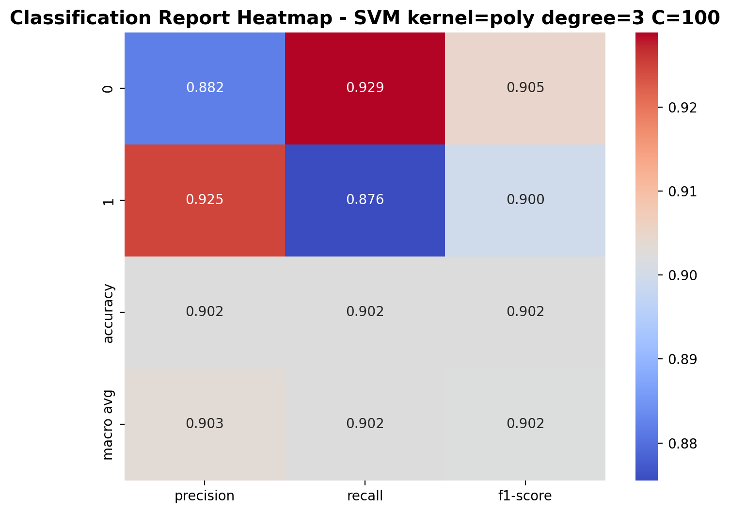
Classification Report - Polynomial Kernel C=100

With C=100, the polynomial kernel SVM achieves good performance. For class 0 (laughter), precision is 0.882, recall is 0.929, and F1-score is 0.905. For class 1 (footsteps), precision is 0.925, recall is 0.876, and F1-score is 0.900. The overall accuracy reaches 90.2%, indicating that increasing the regularization parameter led to diminishing returns.

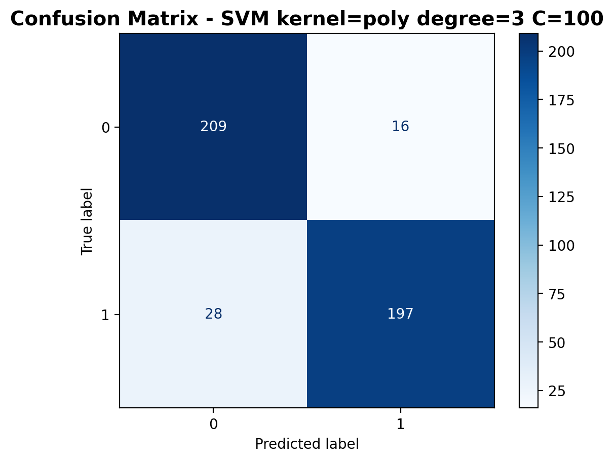
Confusion Matrix - Polynomial Kernel C=100

The confusion matrix shows good performance with 209 correctly classified laughter samples and 197 correctly classified footstep samples. Misclassifications have decreased to 16 laughter samples predicted as footsteps and 28 footstep samples predicted as laughter.

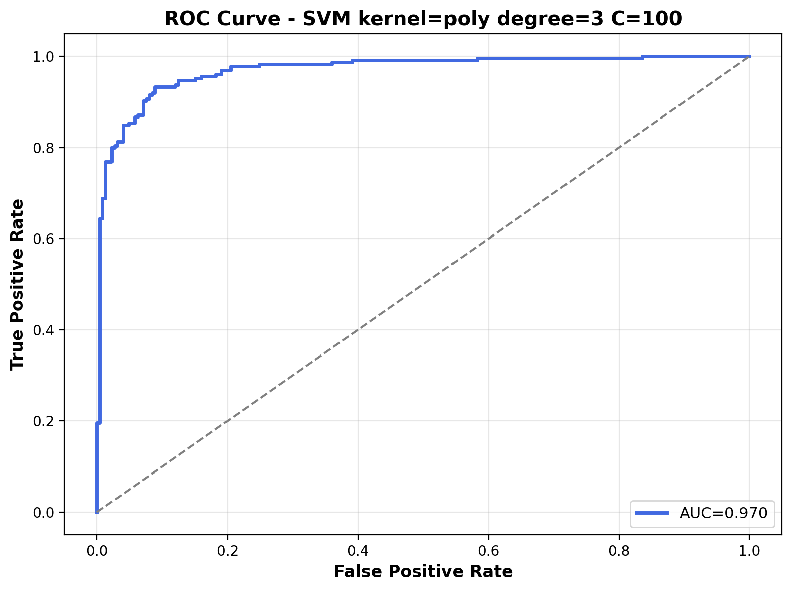
The ROC curve shows great discriminative ability with an AUC of 0.970. The curve approaches the top-left corne, indicating that the polynomial kernel with C=100 achieves excellent separation between the two audio classes across various probability thresholds.

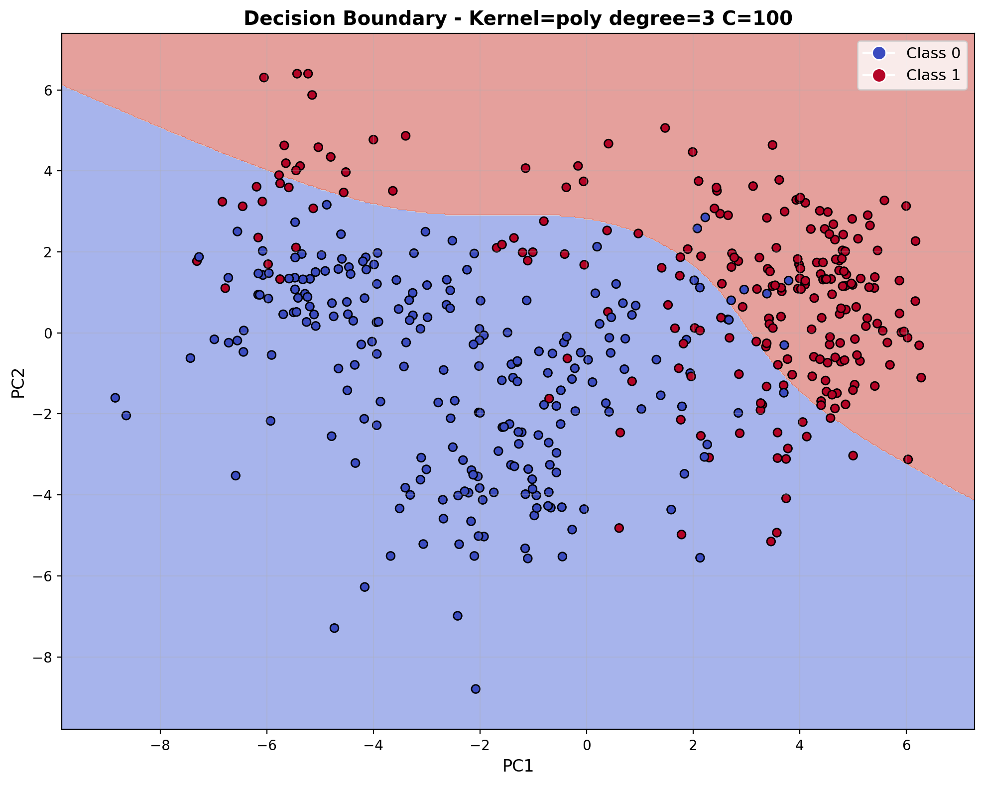
Decision Boundary - Polynomial Kernel C=100

The decision boundary visualization for the polynomial kernel (degree=3) with C=100 displays characteristic curved shapes with smooth transitions throughout the feature space. The boundary forms polynomial curves that separate the audio classes with moderate complexity, creating rounded regions that follow the underlying data distribution. This mathematical structure enables the model to capture non-linear relationships and feature interactions present in the audio data.

Comparison of SVM Models

After evaluating nine different SVM configurations with varying kernels and regularization parameters, a clear pattern emerges regarding their effectiveness for audio classification. The following table summarizes the results across all models:

Kernel	C Value	Accuracy (%)	F1-Score (Class 0)	F1-Score (Class 1)
Linear	0.5	92.4	0.924	0.925
Linear	10	93.1	0.931	0.932
Linear	100	92.9	0.928	0.930
Polynomial (d=3)	0.5	89.3	0.900	0.885
Polynomial (d=3)	10	91.1	0.914	0.908
Polynomial (d=3)	100	90.2	0.905	0.900
RBF	0.5	92.9	0.930	0.927
RBF	10	94.2	0.943	0.942
RBF	100	94.2	0.943	0.941

Key insights from this comparison include:

Kernel Performance: The RBF kernel performs best, especially at higher C values, followed closely by the linear kernel. The polynomial kernel shows lower performance across all regularization parameters. This suggests that while the audio feature space contains non-linear relationships that benefit from the RBF kernel, the feature space may be relatively well-structured as linear kernels also perform effectively.
Regularization Impact: For RBF and linear kernels, increasing the regularization parameter C from 0.5 to 10 provides notable performance improvements. Further increasing to C=100 maintains similar performance or shows slight decreases, indicating an optimal point around C=10.
Model Complexity: Unlike the typical performance ranking often seen in other domains, in this audio classification task, the performance ranking is RBF > Linear > Polynomial. This unexpected pattern suggests that the polynomial kernel may be creating overly complex decision boundaries that don't generalize as well for this specific audio data.
Class Balance: The F1-scores for both classes are remarkably similar across most models, indicating well-balanced class performance. This suggests the models are equally effective at classifying both audio categories.
Optimal Configuration: The RBF kernel with C=10 emerges as the optimal choice, achieving the highest accuracy (94.2%) with more efficient computation compared to C=100, which offers no performance improvement.

Conclusion

Support Vector Machines proved highly effective for audio classification tasks, with the best configuration (RBF kernel, C=10 or C=100) achieving 94.2% accuracy. This analysis demonstrates several key insights:

RBF kernels perform best, but linear kernels deliver surprisingly strong results (93.1%), suggesting the audio features have good linear separability.
The polynomial kernel consistently underperforms both alternatives for this specific audio data.
Optimal performance occurs at moderate regularization (C=10), with minimal improvement at higher values.
Balanced F1-scores across classes indicate effective classification without bias toward either category.

These findings suggest that RBF kernels with moderate C values should be the starting point for audio classification, with linear kernels as an efficient alternative offering strong performance with lower computational requirements. The results highlight the importance of appropriate kernel selection and hyperparameter tuning in SVM applications.

The full script to perform SVM classification, including preprocessing and visualizations, can be found here.

Ensembles

Overview

Ensemble methods are powerful machine learning techniques that combine multiple individual models to create a more robust, accurate, and stable predictive system. The core principle behind ensemble methods is that a group of "weak learners" can come together to form a "strong learner." By aggregating the predictions of several base estimators, ensemble methods reduce variance (bagging), bias (boosting), or improve predictions (stacking). This collective decision-making approach often outperforms any single model, as it mitigates the weaknesses of individual models and harnesses their combined strengths.

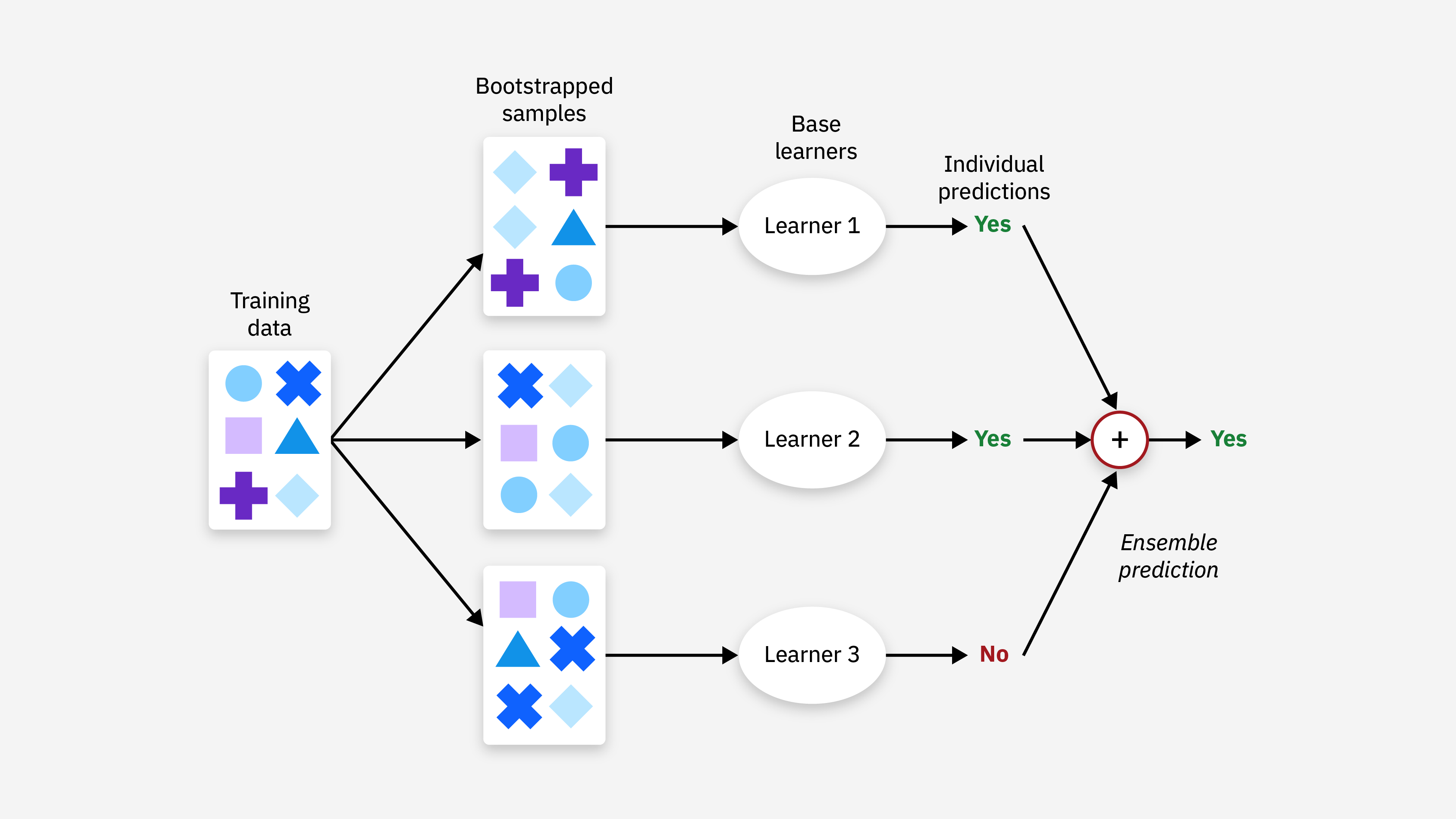
This illustration demonstrates the fundamental concept of ensemble methods. Multiple individual models (weak learners) are trained on different subsets of data or features. Their predictions are then combined through various strategies like voting, averaging, or weighted aggregation to produce a final prediction that is typically more accurate and robust than any single model's prediction.

Ensemble methods can be categorized into several main types:

Bagging (Bootstrap Aggregating): Trains multiple instances of the same learner on random subsets of the training data and aggregates their predictions. Random Forest is a prominent example of a bagging ensemble.
Boosting: Builds models sequentially, with each new model focusing on correctly classifying examples that previous models misclassified. AdaBoost, Gradient Boosting, and XGBoost are popular boosting algorithms.
Stacking: Combines predictions from multiple models using another model as a meta-learner, which learns how to best combine the base models' predictions.
Voting: Simple ensembles that combine predictions from multiple models through majority voting (for classification) or averaging (for regression).

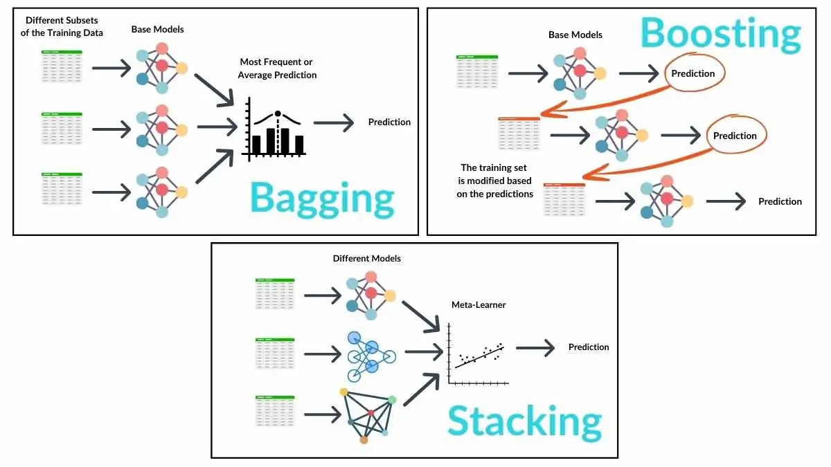
This visualization compares different ensemble techniques. The left panel shows bagging, where models train on bootstrap samples and make independent predictions that are averaged. The right panel illustrates boosting, where models learn sequentially with each model focusing on previously misclassified samples. The bottom panel shows stacking, where predictions from multiple base models become inputs to a meta-model that produces the final prediction.

Random Forest Classifier

Random Forest is a popular ensemble learning method that operates by constructing multiple decision trees during training and outputting the class that is the mode of the classes (for classification) or mean prediction (for regression) of the individual trees. It was developed by Leo Breiman and Adele Cutler, and combines the concepts of bagging (bootstrap aggregation) with random feature selection to create a powerful and versatile algorithm.

The core principles that make Random Forests effective include:

Bootstrap Sampling: Each tree in the forest is trained on a random sample of the training data, drawn with replacement (bootstrap sampling). This introduces diversity among the trees and helps prevent overfitting.
Random Feature Selection: When splitting a node, only a random subset of features is considered. This further decorrelates the trees and makes the ensemble more robust.
Tree Diversity: The combination of bootstrap sampling and random feature selection ensures that each tree in the forest is different, capturing unique patterns in the data.
Voting Mechanism: For classification, the final prediction is determined by majority voting across all trees, while for regression, it's the average of individual tree predictions.

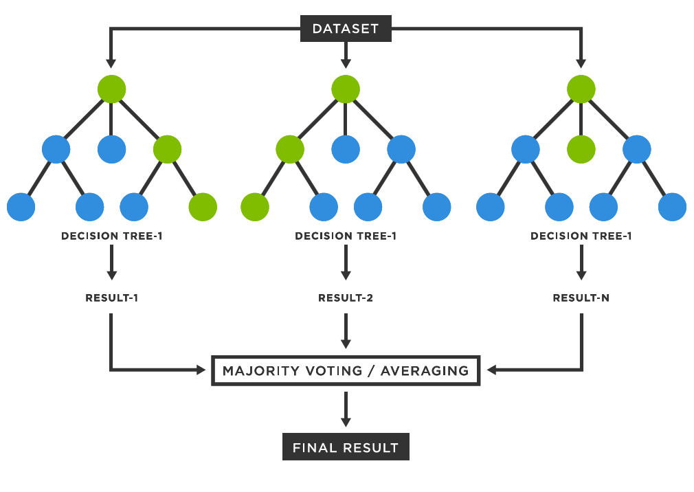
This illustration shows how a Random Forest classifier works. Multiple decision trees are trained on different bootstrap samples of the training data, with each tree considering only a random subset of features at each split. For classification tasks, the final prediction is determined by majority voting across all trees in the forest.

Random Forest Classification of Audio Data

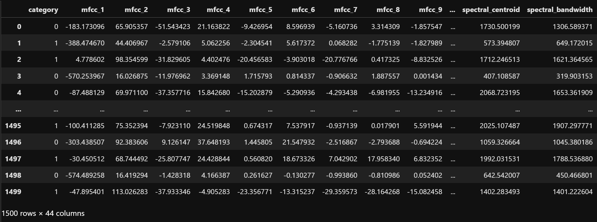
To apply Random Forest to audio classification, a dataset consisting of audio features from two categories is selected: "speech" and "crowd_noise". This binary classification task provides a clear benchmark for evaluating the Random Forest algorithm's effectiveness in distinguishing between different audio types. The dataset for random forest classification is shown below.

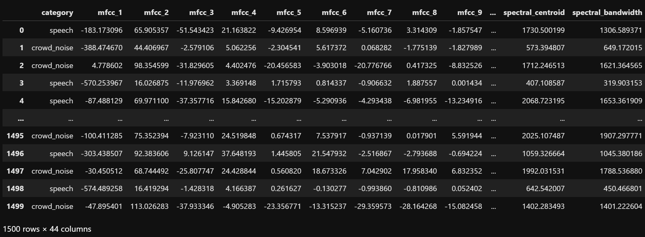
The dataset contains extracted audio features for both "speech" and "crowd_noise" categories. Each row represents one audio sample, with columns corresponding to various audio features like spectral contrast, MFCCs, chroma, and other acoustic descriptors used for classification.

For the classification task, the categories are encoded as binary values: "speech" as 0 and "crowd_noise" as 1. This encoded dataset serves as the foundation for the Random Forest model. The encoded dataset is shown below.

The dataset after binary encoding of categories. The "category" column now contains numeric values (0 for "speech", 1 for "crowd_noise") suitable for machine learning algorithms.

The dataset is split into training (70%) and testing (30%) sets using stratified sampling to maintain class distribution. The training and testing sets are shown below.

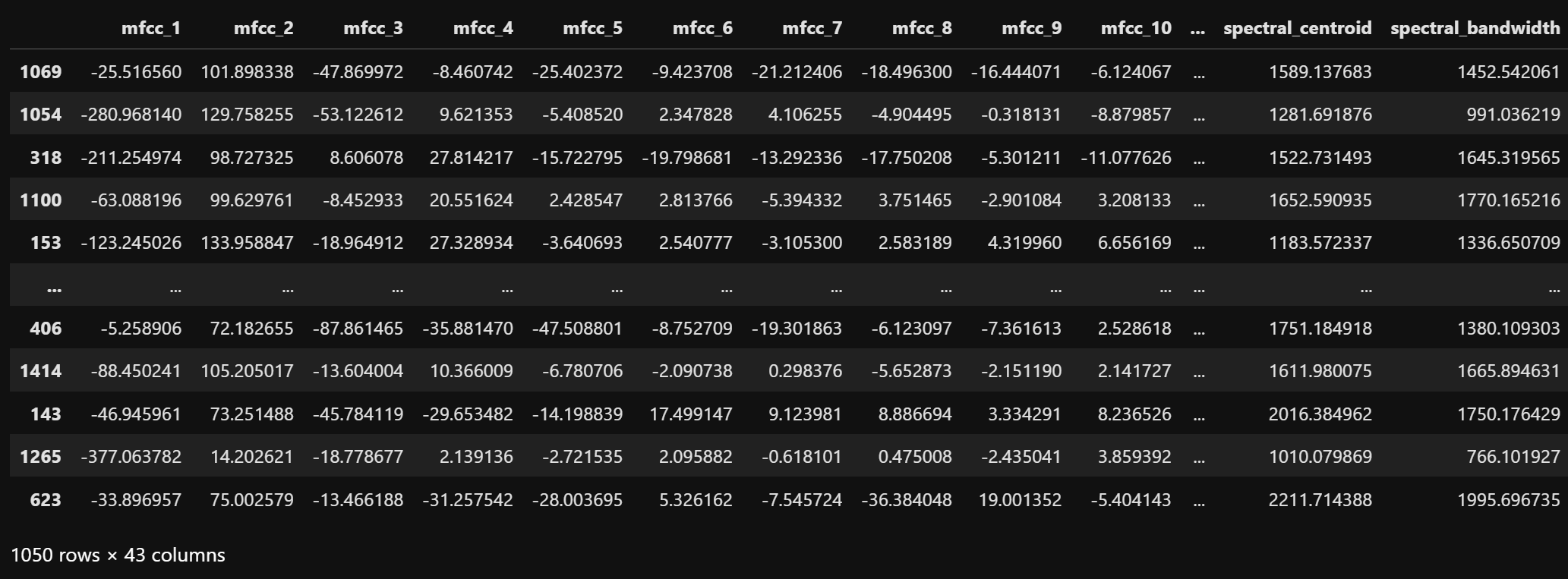
The training dataset contains 70% of the original samples, maintaining the same class distribution. This set is used to train the Random Forest classifier.

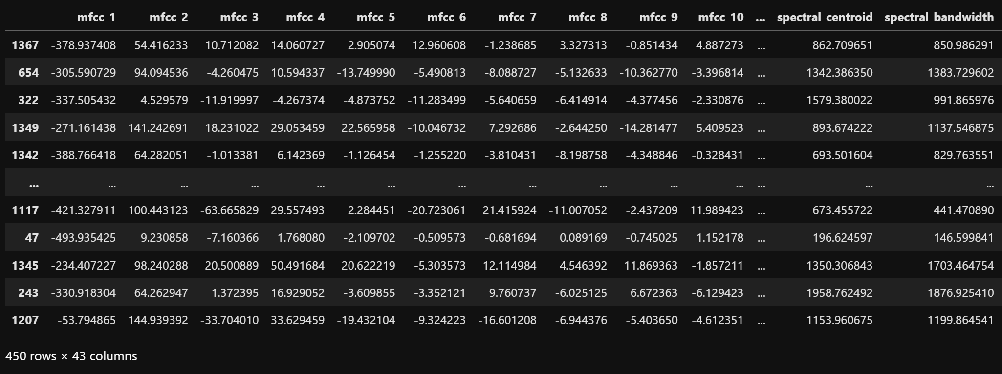
The testing dataset contains the remaining 30% of samples and is used to evaluate model performance on unseen data.

Implementing Random Forest Classification

For this audio classification task, a Random Forest classifier with default parameters is implemented. The implementation uses scikit-learn's RandomForestClassifier with a fixed random seed for reproducibility. Random forest classifier is a tree based model and does not require any feature scaling. So the train and test sets are used directly here. The model is evaluated on the test set using multiple metrics including accuracy, precision, recall, F1-score, confusion matrix, and area under the ROC curve (AUC).

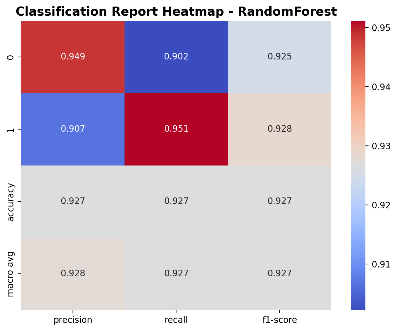
The classification report shows the performance metrics for the Random Forest classifier. For class 0 (speech), the model achieved a precision of 0.949, recall of 0.902, and F1-score of 0.925. For class 1 (crowd_noise), the precision was 0.907, recall was 0.951, and F1-score was 0.928. The overall accuracy is 92.7%, with similar macro-average metrics, indicating balanced performance across both classes.

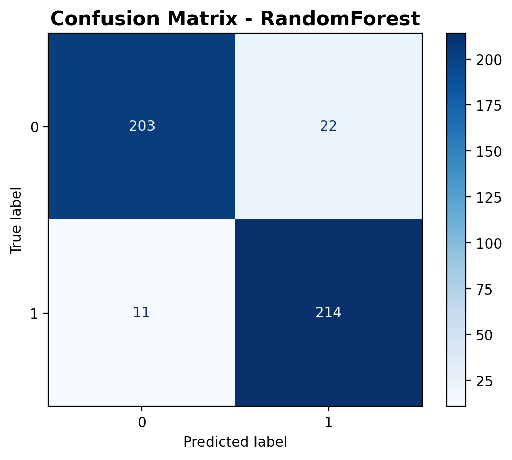
The confusion matrix provides a detailed breakdown of predictions. The model correctly classified 203 speech samples and 214 crowd noise samples, while misclassifying 22 speech samples as crowd noise and 11 crowd noise samples as speech. This visualization helps understand where the model makes errors and whether it has any bias toward a particular class.

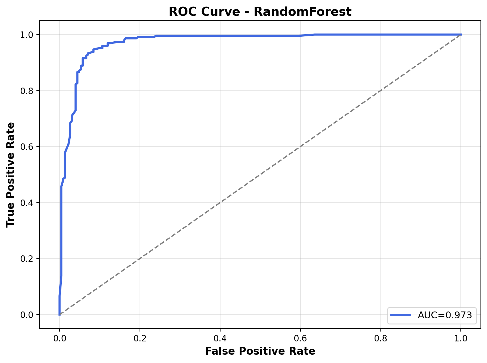
The ROC curve illustrates the model's performance across different classification thresholds. The Area Under the Curve (AUC) is 0.973, indicating excellent classification performance. The curve's proximity to the top-left corner reflects the model's ability to differentiate between speech and crowd noise with high confidence.

Conclusion

The Random Forest classifier demonstrated strong performance in distinguishing between speech and crowd noise audio, achieving an accuracy of 92.7% and an AUC of 0.973. These results highlight key insights:

The ensemble approach effectively captures complex audio patterns, leading to high classification accuracy.
Balanced F1-scores (0.925 for speech, 0.928 for crowd noise) indicate no significant bias toward either class.
The high AUC of 0.973 shows the model's strong ability to distinguish between audio categories across different thresholds.
Random Forest’s feature selection capability identifies the most informative audio features without needing explicit scaling or normalization.

These findings suggest that Random Forest is highly effective for audio classification tasks, handling high-dimensional feature spaces with minimal preprocessing or tuning.

The complete script for Random Forest classification, including data preparation and visualizations, is available here.