Data Preparation & Exploration
Data Collection: Gathering Audio Data Using the Freesound API
For this project, a diverse set of environmental and everyday sounds was collected using the Freesound API, a public database of user-contributed audio recordings. The API provides a structured way to search, filter, and retrieve metadata for various sound categories, making it an ideal source for curating a dataset for machine learning analysis.
Using the Freesound API
Accessing the Freesound API requires an API key, which can be obtained by signing up on the Freesound website. The API enables users to search for sounds based on keywords and retrieve detailed metadata before downloading the corresponding audio files. The data collection process began by querying the API for relevant sound clips and extracting their metadata, which was then used to facilitate audio file downloads. Get a freesound API here.
Selecting 20 Sound Categories
To ensure a balanced dataset covering a range of real-world sounds, 20 categories were carefully selected.
The selection process focused on sounds commonly found in various environments, including human, animal, instrumental, and environmental sounds.
Each category was chosen to provide clear, recognizable acoustic patterns that could be effectively analyzed and classified.
The final 20 categories in the dataset include:
- Human-related sounds: applause, crowd_noise, laughter, speech
- Animal sounds: birds, cat_meow, dog_bark
- Instrumental sounds: drums, guitar, piano
- Environmental and urban sounds: rain_sounds, wind_sounds, thunder_sounds, traffic_sounds, train_sounds, sirens
- Mechanical and impact sounds: car_horn, footsteps, fireworks, construction_noise
For consistency, the target was to collect 750 sound samples per category. However, due to data limitations, only 687 car_horn sounds were available in the Freesound database.
Retrieving Metadata and Downloading Audio Files
Before downloading the audio files, their metadata was first collected using the Freesound API. Each API query returned a JSON file containing essential details for each sound, including:
- Sound ID
- Name
- Tags
- Duration
- Preview URL (link to download a short version of the sound)
- License Information
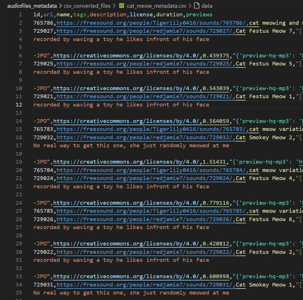
After downloading the metadata JSON files, they are converted to CSV files for ease of handling. They are also checked for any missing or repeated values. No repeated or missing values were found. Check out the script to download audiofiles metadata using Freesound API and convert them to CSV files here. The raw metadata JSON files can be found here and the converted csv files can be found here.
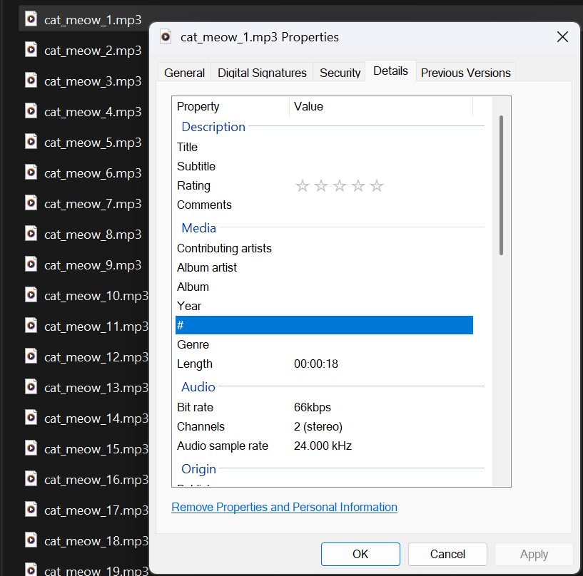
Once the metadata JSON files were obtained, the preview URLs provided in the metadata were used to download the audio files. The downloads were executed in parallel using multi-threading to optimize efficiency and speed. Check out the script to download audio files here. The downloaded audio files are in .mp3 format. The downloaded raw audio files can be found here.
The raw metadata JSON files and the raw audio mp3 files for any category look like the ones shown below.
Raw Metadata JSON

Raw .mp3 Audio files
Data Preprocessing: Conversion and Standardization of Audio Data
After collecting the raw audio files, preprocessing was necessary to ensure consistency across all samples. The dataset contained files of a lossy format with varying durations, sample rates, and amplitudes, requiring standardization before feature extraction and analysis. All audio processing was done using Librosa, a Python library designed for audio analysis. Under the hood, Librosa utilizes FFmpeg to handle audio file decoding and conversion, allowing seamless processing of different formats.
Format Conversion
The downloaded audio files were originally in MP3 format, which is compressed and may lead to loss of audio quality. To ensure high-quality, lossless processing, all files were converted to WAV format. The WAV format was chosen because it preserves full spectral details, making it ideal for machine learning applications.
Duration Standardization (Fixed-Length Audio)
Audio samples in the raw dataset varied significantly in duration, with some clips lasting only a second while others exceeded a minute. To create a uniform dataset, each audio file was trimmed or padded to exactly 5 seconds. The trimming approach was adjusted based on the audio length:
- If a file was longer than 5 seconds, it was trimmed from the middle to preserve core information.
- If a file was shorter than 5 seconds, it was padded with silence equally at the beginning and end to maintain balance.
Mono Channel Conversion
Additionally, all audio files were converted to mono-channel to ensure consistency, as some recordings had multiple channels (stereo). This prevented unwanted variations in feature extraction due to channel differences.
Sample Rate Standardization
Different recordings had varying sample rates (e.g., 44.1 kHz, 22.05 kHz, 16 kHz), which could cause inconsistencies in feature extraction. To standardize all audio files, a sampling rate of 16,000 Hz was applied, ensuring compatibility across all files while keeping sufficient frequency detail for analysis.
Amplitude Normalization
The raw audio files had varying loudness levels, which could introduce bias in classification. Some recordings were significantly louder, while others were barely audible. To address this, each audio waveform was normalized so that amplitudes fell within a consistent range, preventing any single sound from dominating due to volume differences.
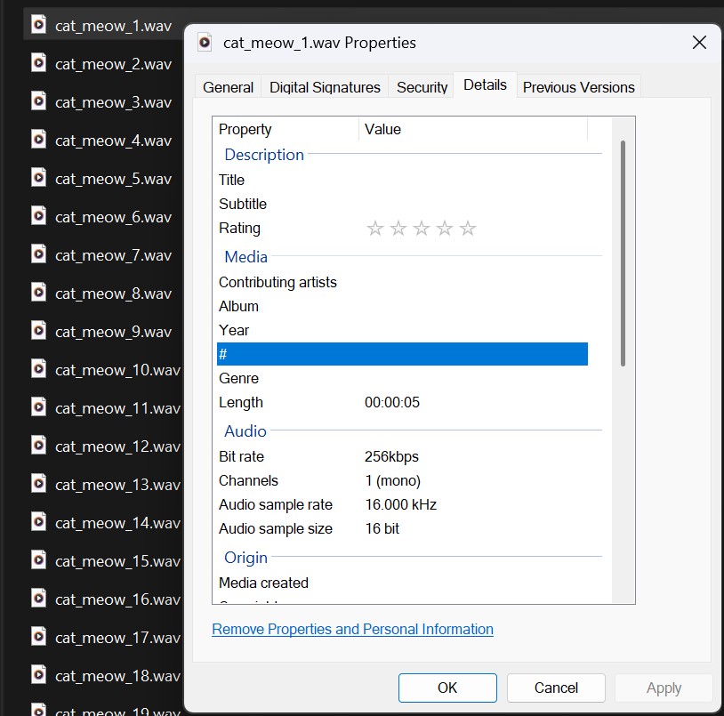
After preprocessing, the script also verified that all files were functional and met the expected duration (5 seconds), sample rate (16 kHz), and mono-channel format before proceeding to feature extraction. The processed .wav audio files can be found here. Check out the full audio files processing script here.
The metadata JSON files were already converted to CSV files and made clean enough by the script downloading them. The converted CSV metadata files and the processed audiofiles for any category look like the ones shown below.
Converted Metadata CSV
Processed .wav Audio files
Feature Extraction: Transforming Audio into Machine-Readable Data
After preprocessing, the next step involved extracting meaningful features from the standardized audio files. Since raw audio waveforms are not directly usable for machine learning, numerical representations of key sound properties were generated. These extracted features capture both temporal and spectral characteristics of each sound, making them suitable for classification and analysis.
Extracted Features
The following features were extracted for each 5-second audio file:
- MFCCs (Mel-Frequency Cepstral Coefficients) – Captures frequency-based characteristics related to timbre
- Chroma Features – Represents the distribution of pitch across musical notes
- Spectral Contrast – Measures the difference between peaks and valleys in the frequency spectrum
- Zero-Crossing Rate (ZCR) – Counts how often the waveform crosses the zero amplitude level
- Spectral Centroid – Indicates the "center of mass" of the frequency spectrum
- Spectral Bandwidth – Measures how spread out the spectral energy is
- RMS Energy (Root Mean Square Energy) – Represents the loudness of the sound
- Spectral Roll-off – The frequency below which most spectral energy is concentrated
- Tonnetz (Tonal Centroid Features) – Captures harmonic and tonal relationships
These features provide a structured way to analyze and classify different sound categories.
Feature Extraction Process
To efficiently process thousands of audio files, Librosa was used to extract features, with parallelization implemented for speed optimization. Each audio file was loaded at a 16,000 Hz sample rate, converted to mono-channel, and analyzed to compute the listed features. The extracted values were averaged over time to create a fixed-length numerical representation for each file.
Storing Extracted Features
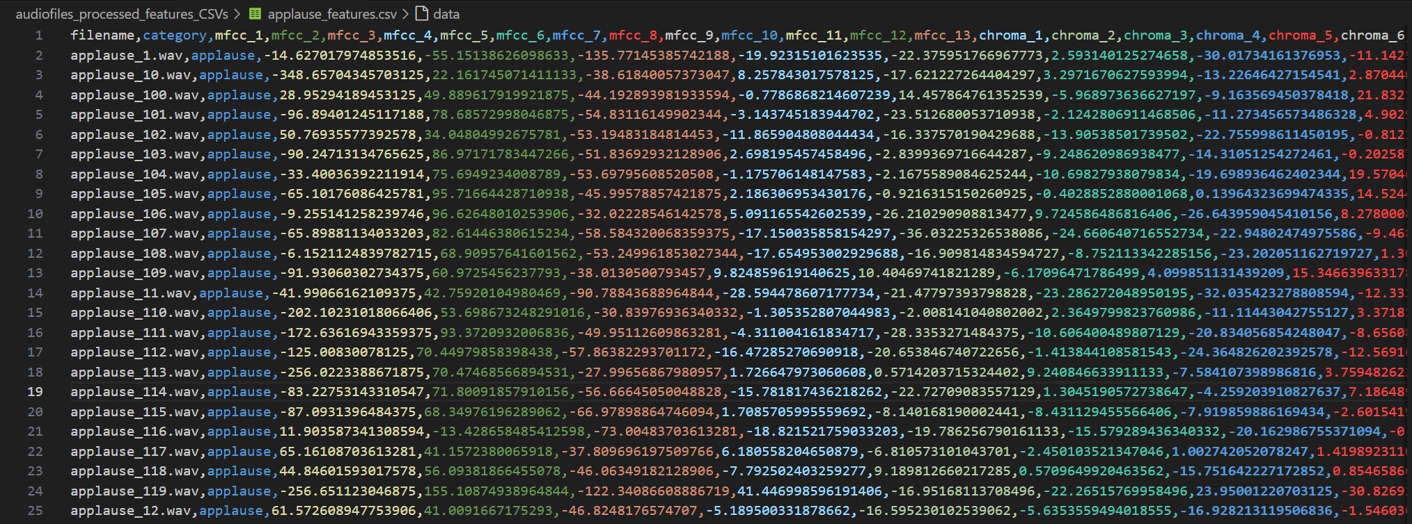
The extracted features were stored in CSV files, with each row representing an audio file and columns containing the corresponding feature values. The CSV structure included:
- Filename for reference
- Category for reference
- 13 MFCC coefficients
- 12 Chroma features
- 7 Spectral contrast values
- Zero-crossing rate
- Spectral centroid
- Spectral bandwidth
- RMS energy
- Spectral Roll-off
- 6 Tonnetz features
This structured dataset allows for further analysis and classification using machine learning techniques. Check out the feature extraction script here.
The Audio Features CSV file for any category looks like the one shown below.
Audio Features CSV
Data Exploration: Visualizing the Sounds
MFCC Radial Plots
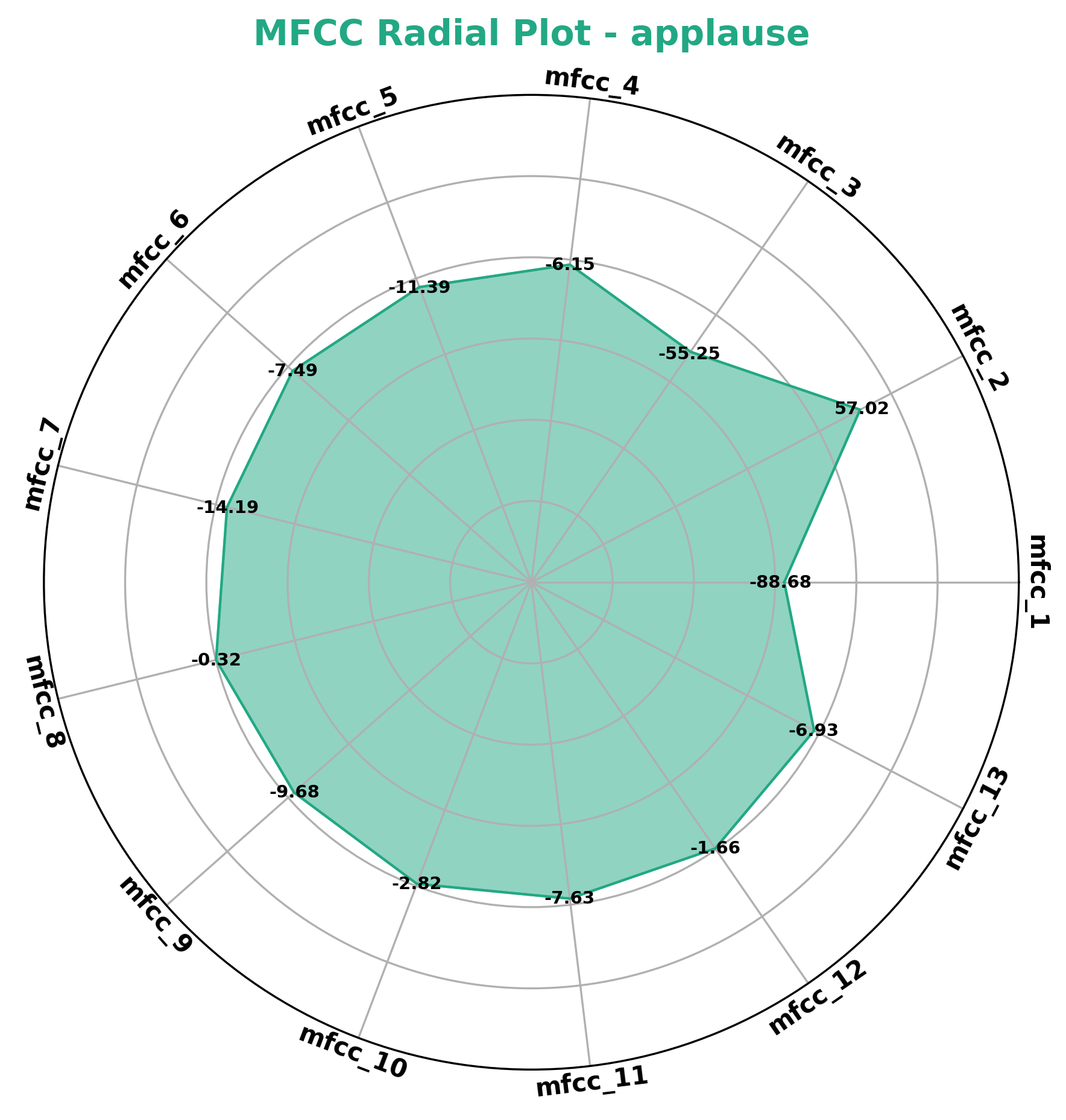
This plot visualizes the Mel-Frequency Cepstral Coefficients (MFCCs) in a circular (spider) plot. MFCCs are used to characterize the spectral properties of audio signals, and the radial plot helps compare how different sound categories distribute their MFCC values.
3D Spectral Feature Plot
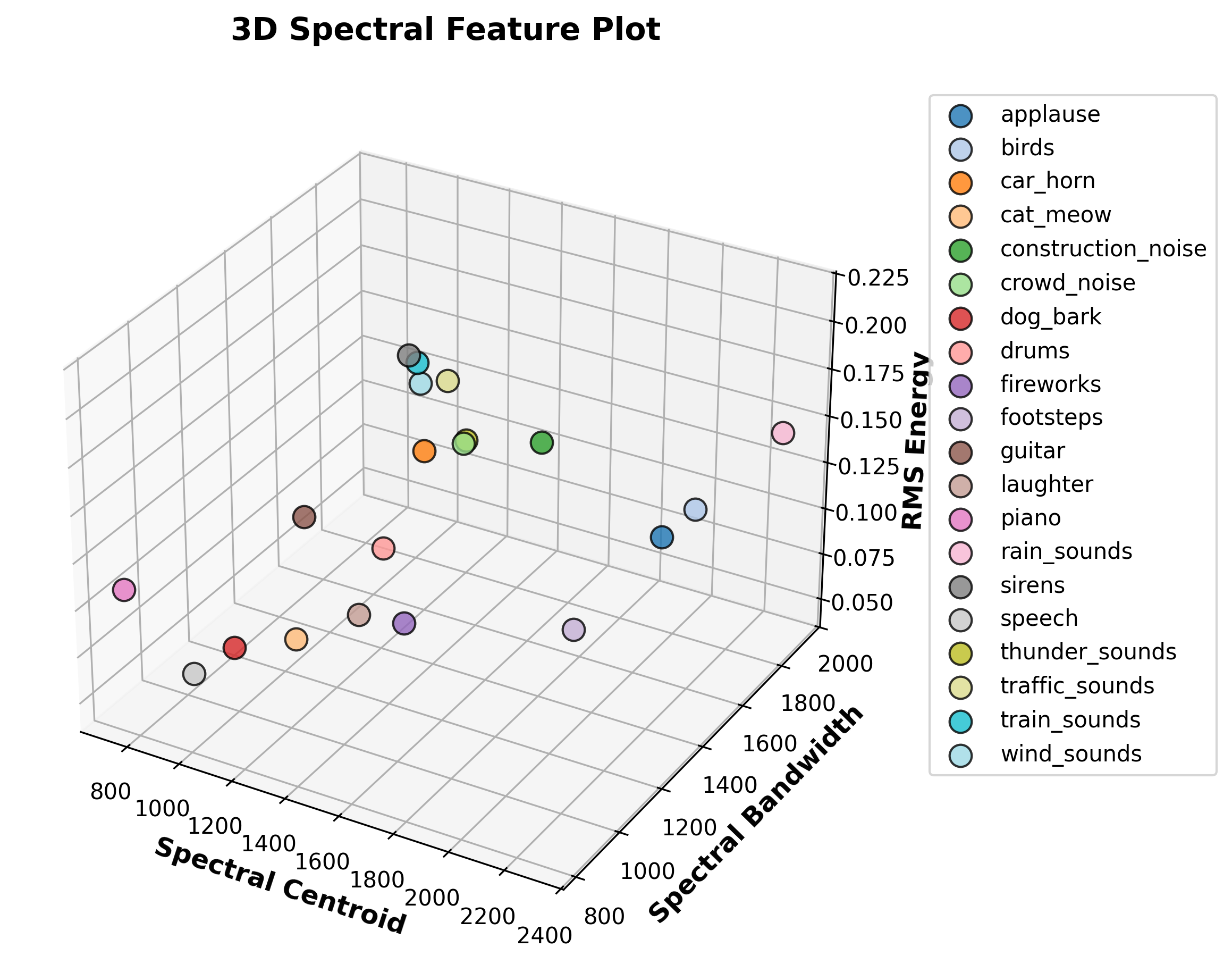
A 3D scatter plot showcasing three key spectral features: Spectral Centroid, Spectral Bandwidth, and RMS Energy. These features provide insights into the brightness, spread, and energy of different audio categories.
Chroma Feature Heatmap
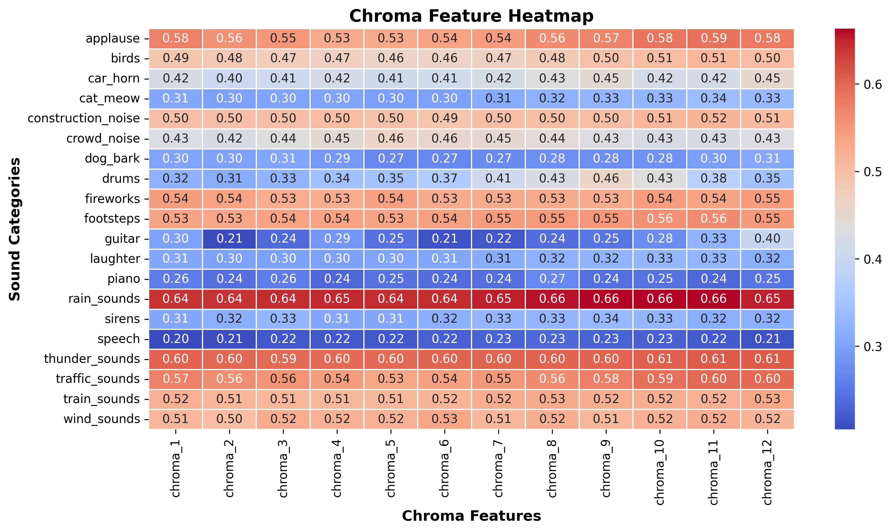
This heatmap displays the average chroma feature values for each sound category. Chroma features capture pitch class distributions and are useful for analyzing tonal characteristics across different sounds.
Average Spectrograms
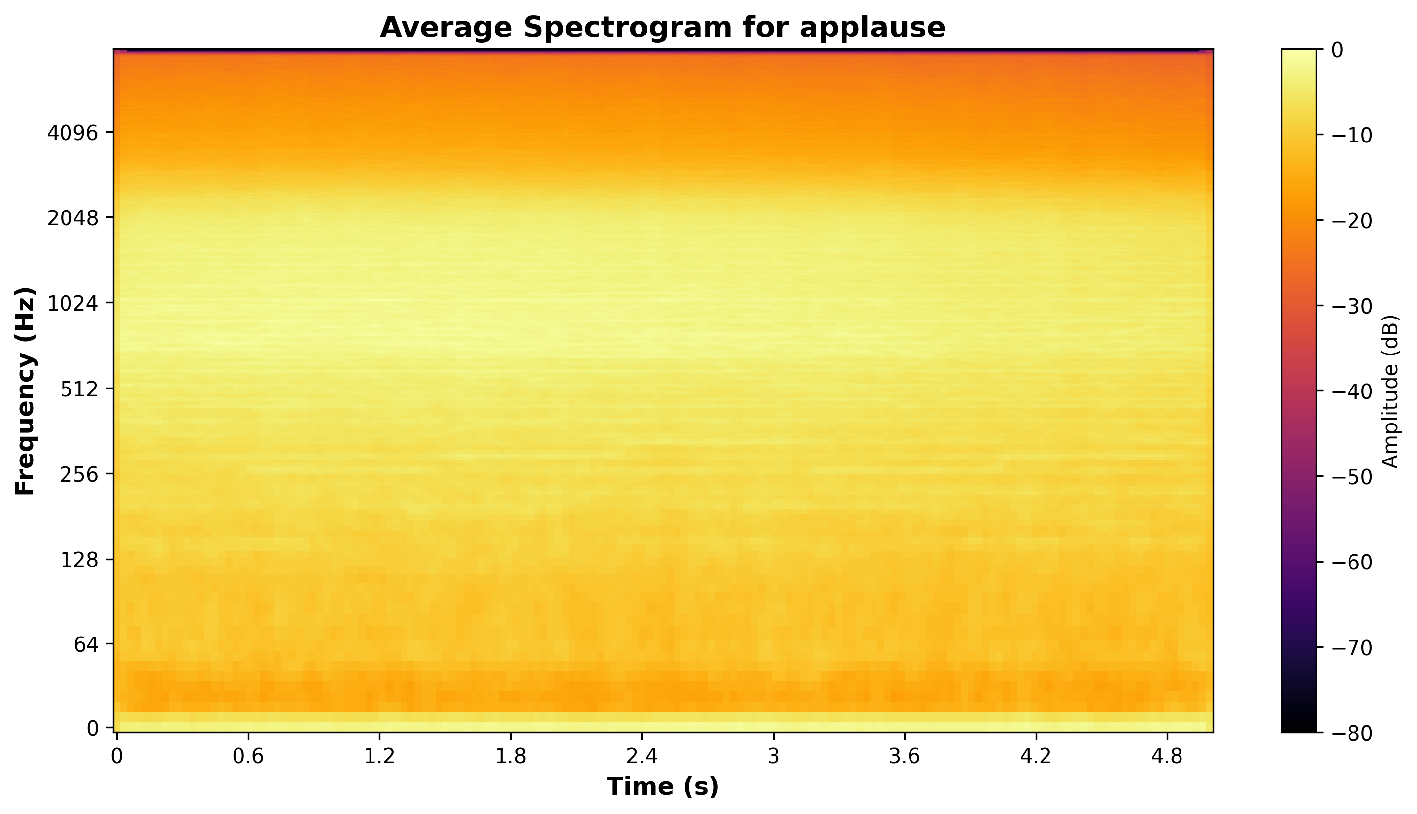
This plot presents an averaged spectrogram for each category, illustrating how frequency content evolves over time. It provides a visual representation of how different sounds occupy the frequency spectrum.
Time-Series Plots of RMS Energy
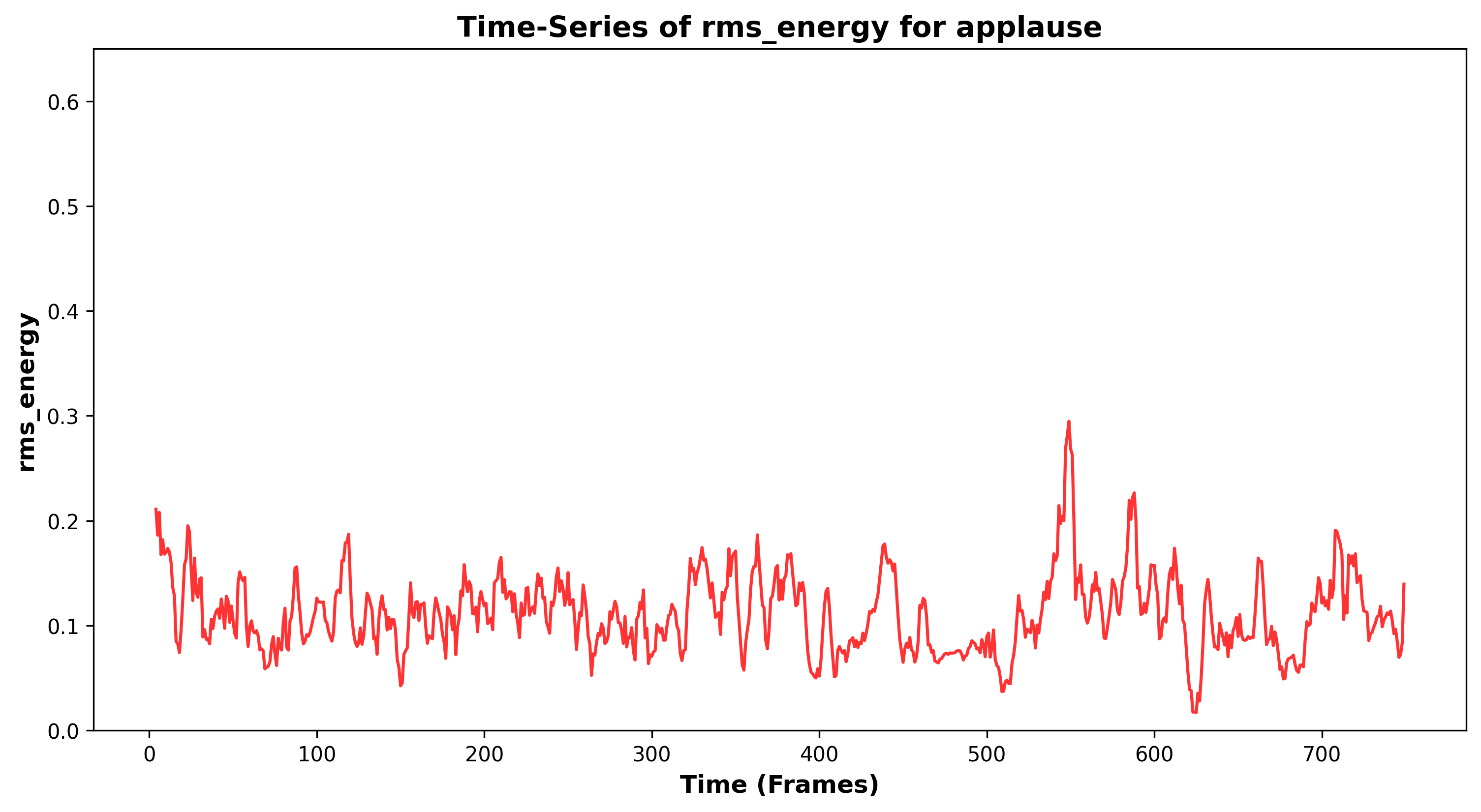
A time-series plot of RMS (Root Mean Square) energy values, representing the loudness variations of different sound categories over time. A rolling average smooths fluctuations to highlight trends.
Zero-Crossing Rate Histograms
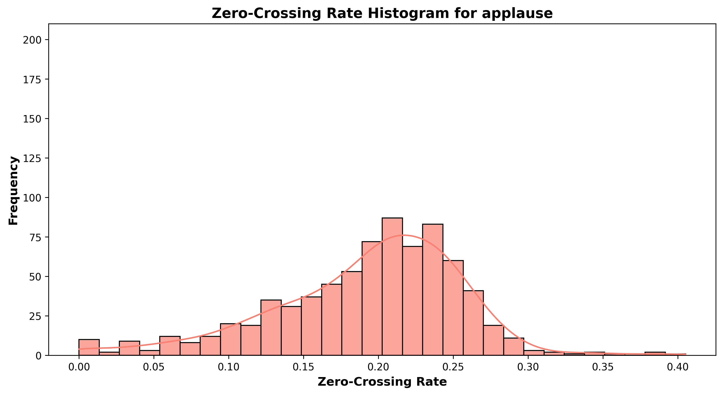
A histogram showing the distribution of zero-crossing rates (ZCR) across sound categories. ZCR measures how frequently the signal crosses the zero amplitude line, making it useful for distinguishing percussive from tonal sounds.
Mean Spectral Contrast
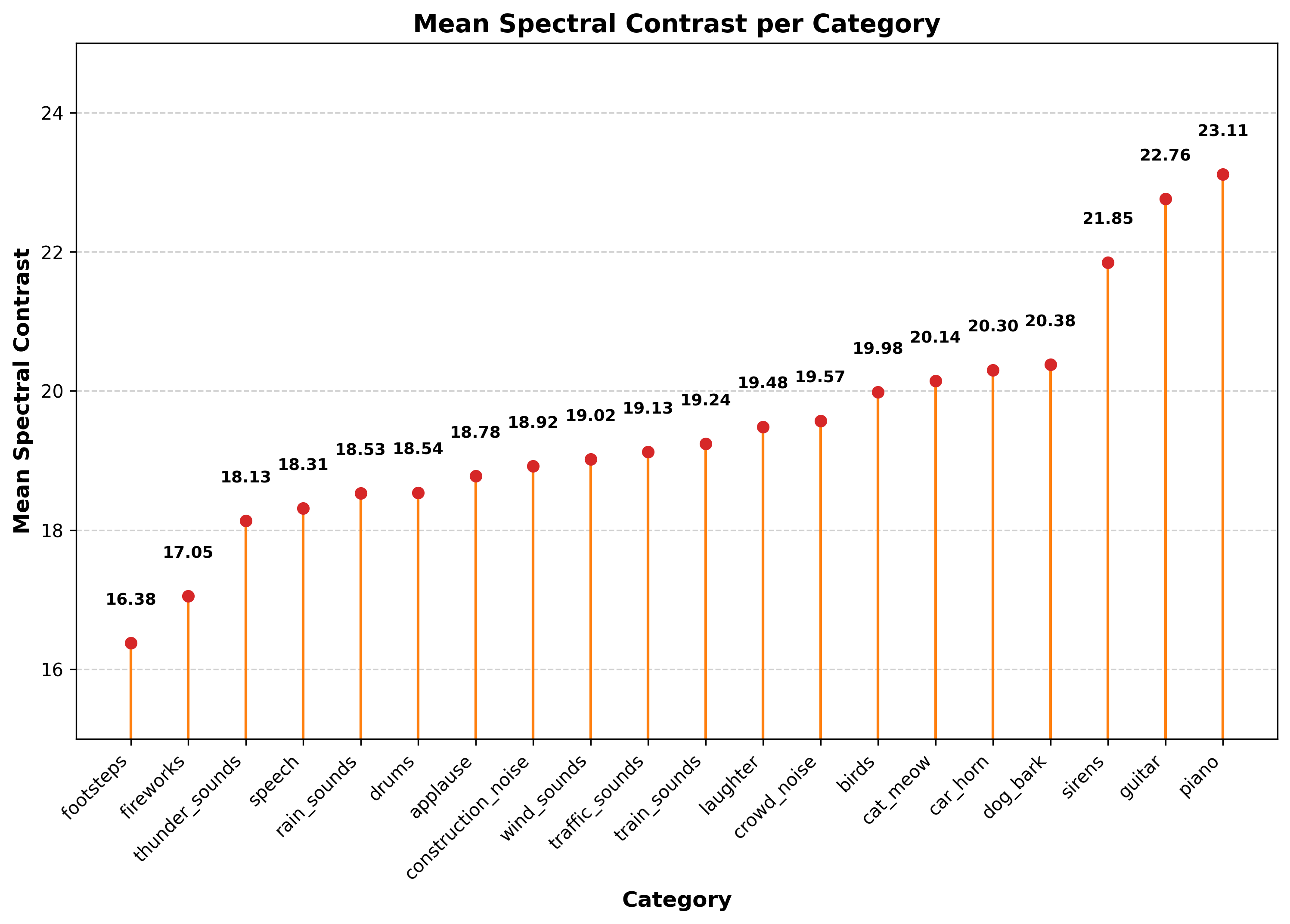
A lollipop chart illustrating the mean spectral contrast per category. Spectral contrast measures the difference between peaks and valleys in a sound spectrum, helping differentiate between tonal and noisy sounds.
Spectral Roll-off Distribution
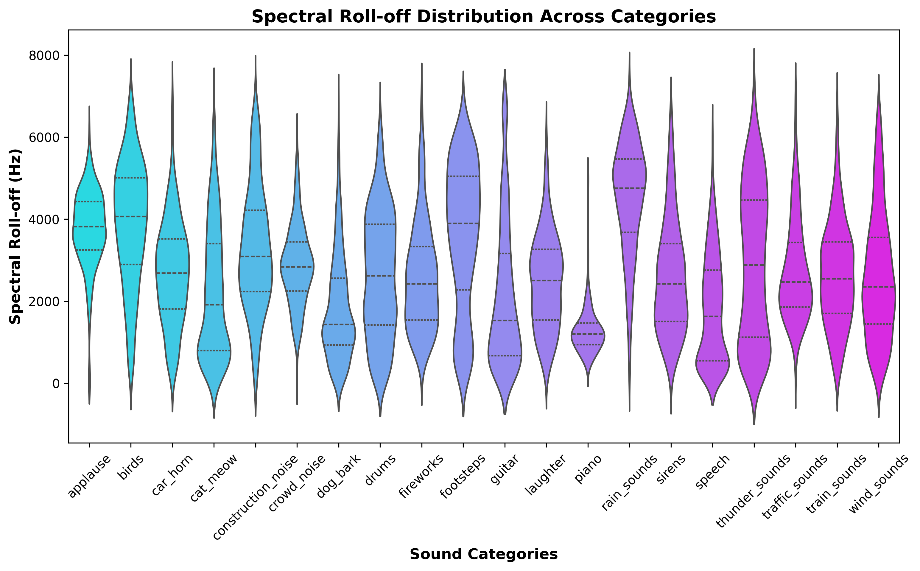
A violin plot showing the distribution of spectral roll-off values for each category. Spectral roll-off represents the frequency below which most of the spectral energy is concentrated, helping identify bright vs. muffled sounds.
Tonnetz Feature Distribution
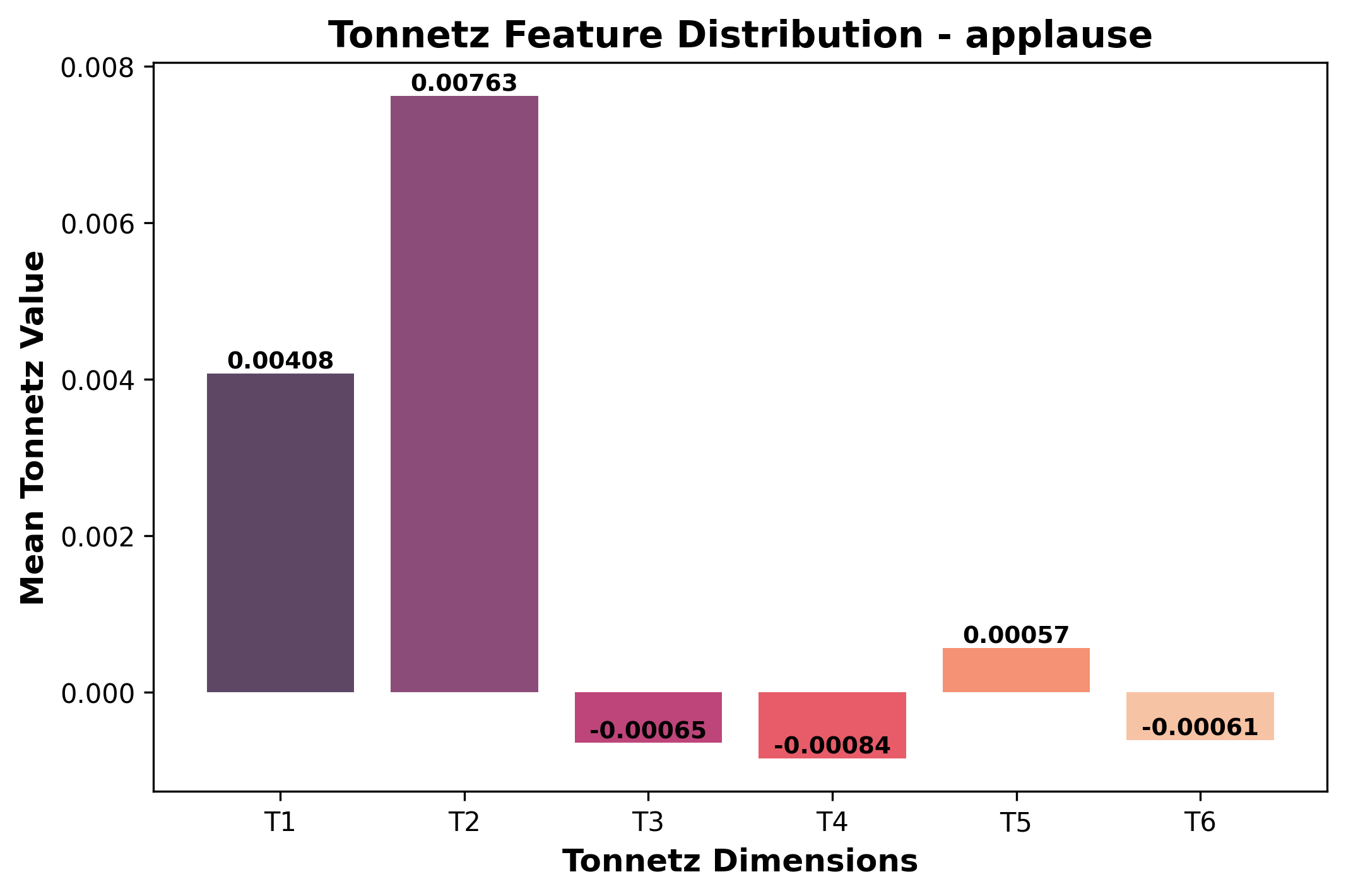
A grouped bar chart displaying the average values of Tonnetz features for each category. Tonnetz features capture harmonic and tonal characteristics, useful for music analysis and tonal sound classification.
Feature Variability Plots
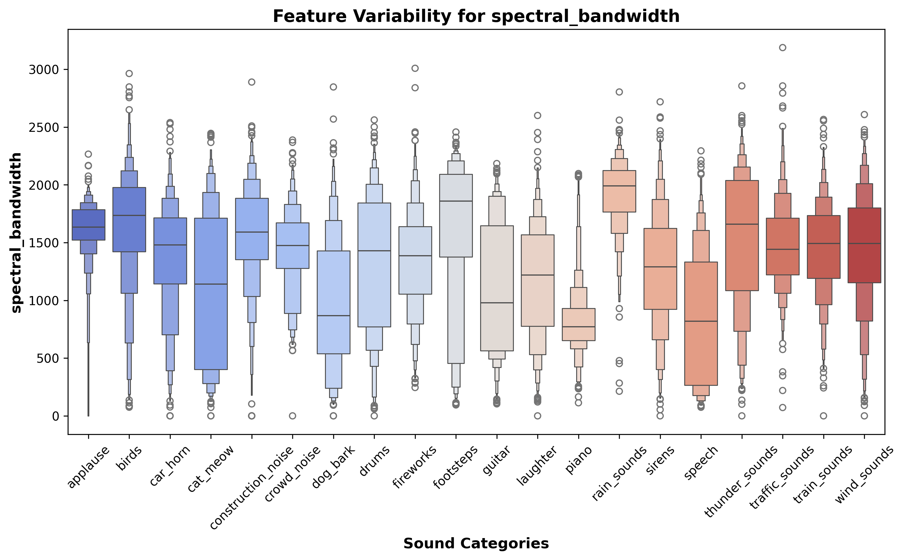
A boxen plot visualizing the variability of selected features (Zero Crossing Rate, Spectral Centroid, Spectral Bandwidth, Rms Energy, Spectral Rolloff) across sound categories. It highlights the range and distribution of feature values.
Check out the full script to create the Visualizations here.